Diff Studio
Differential equations are crucial in modeling complex systems - from pharmacology and drug manufacturing to financial modeling and environmental studies.
Datagrok Diff Studio solves initial value problems for ordinary differential equations (ODEs) and visualizes solutions in real time, turning complex math into interactive visual models.
Key benefits:
- For model users
- Instantly see how parameter changes affect your system
- Find optimal parameter values that match your target data
- Explore model behavior using Monte Carlo, Sobol, and other methods
- For model creators
- Focus on the math - the platform handles visualization and interface
- Start quick with pre-built models
- Solve both stiff and non-stiff equations
- Handle complex multi-equation ODE systems
- Debug equations easily
- For organizations
- Store and share all ODE models in one, centralized hub
- Convert models to scripts to extend functionality or integrate with other Datagrok tools
- Build specialized scientific applications
Working with models
Launch Diff Studio from Apps > Diff Studio. The app opens with your recent model, or a default template if it's your first time.
To load an existing model, click the Open icon and choose:
- Import... to import local IVP files (or simply drag-and-drop)
- Library to open a production model from the catalog
- Templates to start with a model template
- My Models to open a model from your platform files (Browse > Files > My files)
- Recent to open your recent models
Once loaded, explore models by adjusting parameters, fitting to experimental data, or running sensitivity analysis. Share specific model runs by copying and sharing the URL with colleagues.
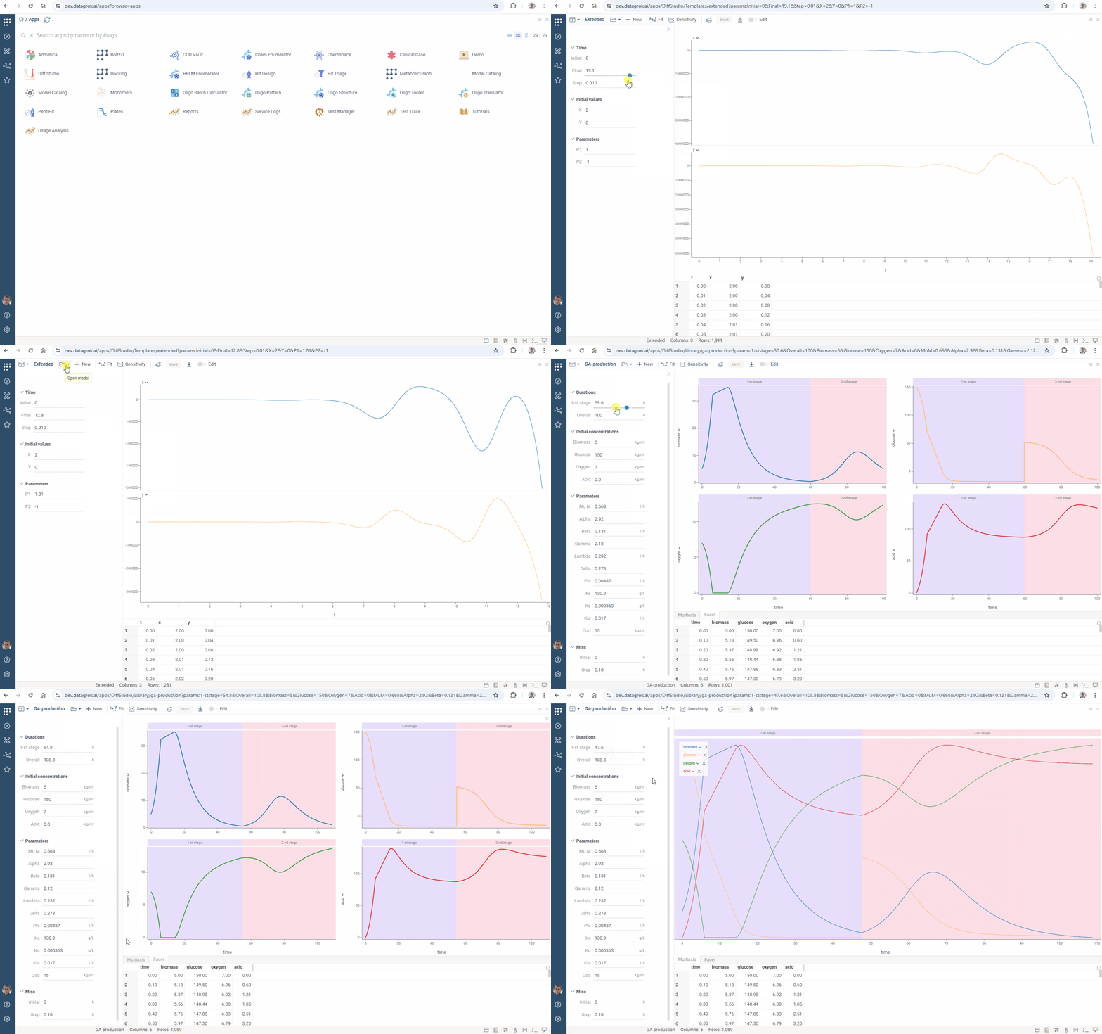
Download models using the Download icon as IVP files, which you can edit in any text editor. To store a model in Datagrok, click the SAVE button and specify the location.
Analyze your model:
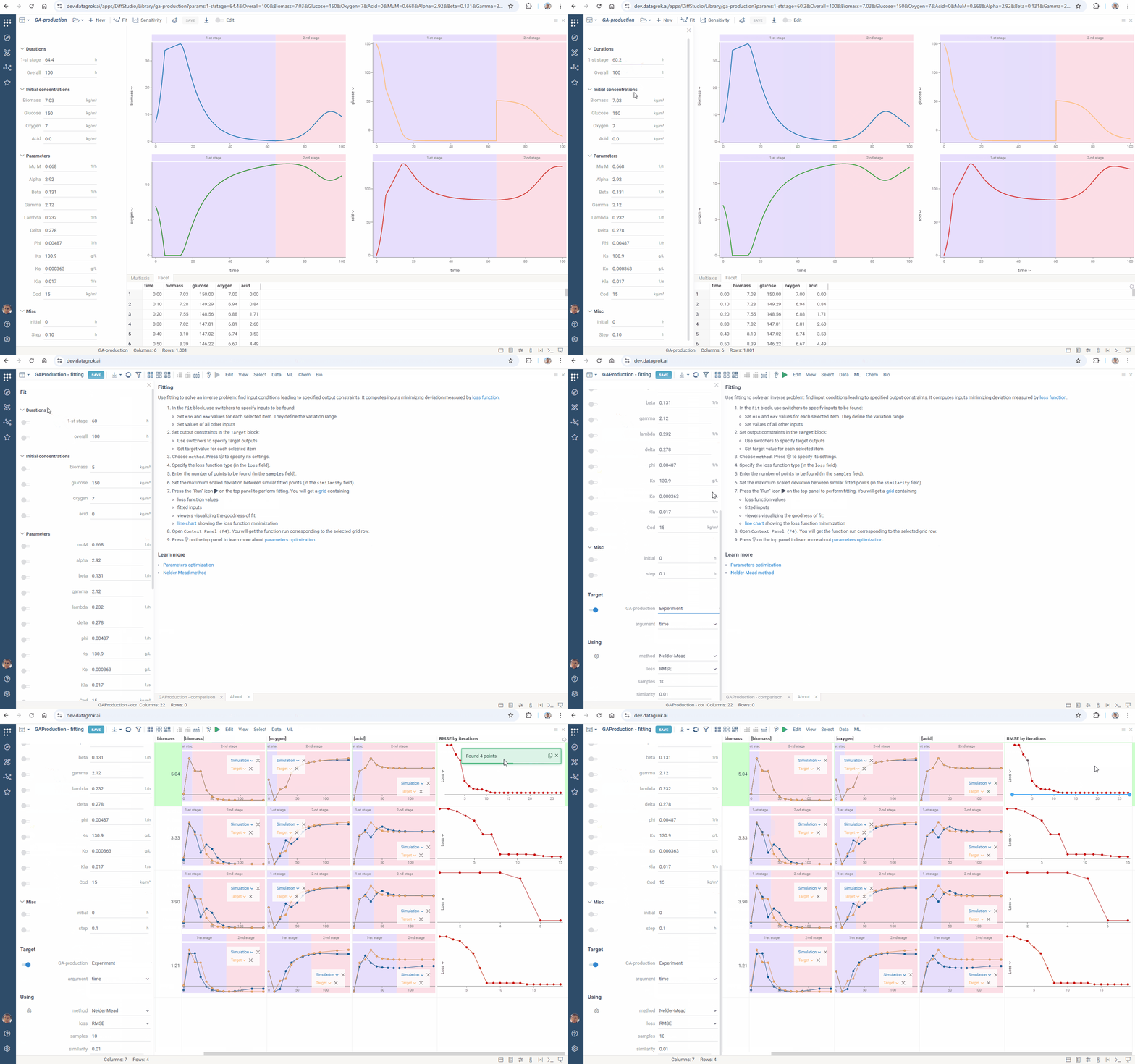
- Parameter Optimization: Click the Fit icon on the top panel to find input conditions that satisfy output constraints.
- Sensitivity Analysis: Click the Sensitivity icon to explore the relationship between inputs and outputs of your model.
Creating models
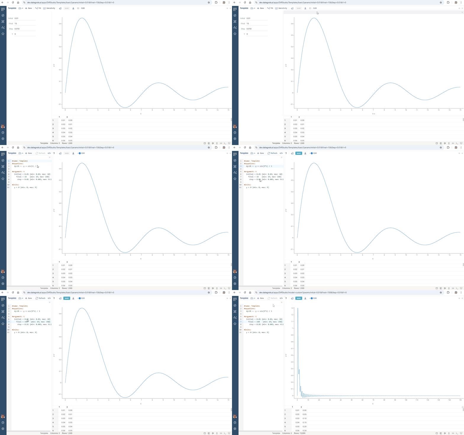
Turn on the Edit toggle on the top panel. Equations editor opens. Edit formulas or add new ones. Click Refresh or press F5 to apply changes.
Model components and syntax
Core blocks
These blocks define the basic mathematical model and are required for any model:
-
#name: Add a model identifier#name: Problem 1 -
#equations: Define the system of ODEs to solve. Diff Studio supports any number of equations with single or multi-letter variable names#equations:dx/dt = x + y + exp(t)dy/dt = x - y - cos(t) -
#argument: Defines- independent variable
- its initial value (
initial) - final value (
final), and - grid step (
step)
The solver calculates values at each step interval across the specified [initial,final] range.
#argument: tinitial = 0final = 1step = 0.01 -
#inits: Defines initial values for functions being solved#inits:x = 2y = 5
Comments
-
#comment: Write a comment in any place of your model#comment:You can provide any text here. Diff Studio ignores it. -
Place comments right in formulas using
//#equations:dx/dt = x + y + exp(t) // 1-st equationdy/dt = x - y - cos(t) // 2-nd equation
Model parameters
These blocks define values used in equations. Choose type based on intended use:
-
#parameters: Generate UI controls for model exploration#parameters:P1 = 1P2 = -1 -
#constants: Use for fixed values in equations that don't require UI controls#constants:C1 = 1C2 = 3
Auxiliary calculations
This block defines mathematical functions using #parameters, #constants,
#argument, and other functions. These are direct calculations (no ODEs involved). Use them to break
down complex calculations and simplify your equations.
-
#expressions#expressions:E1 = C1 * t + P1E2 = C2 * cos(2 * t) + P2
Advanced features
These blocks enable simulations for complex processes.
Cyclic processes
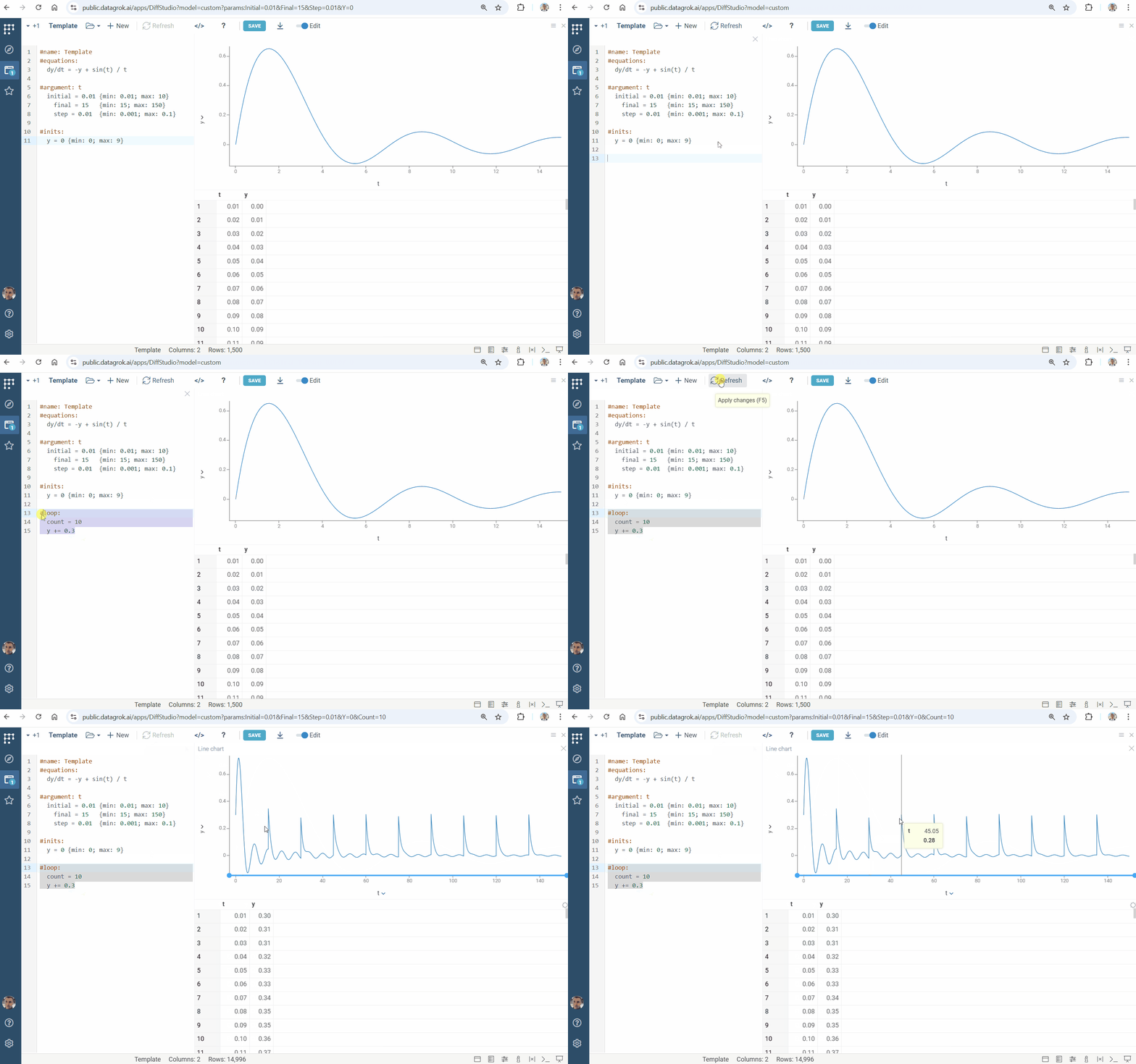
Use the #loop block for cyclic processes. Set count for number of cycles and use any valid mathematical expressions to modify parameters and functions. You can set new values for parameters and change values for functions.
#equations:
  dy/dt = -y + sin(N*t) / t

#parameters:
  N = 1

#loop:
  count = 3
  N += 2
Multistage processes
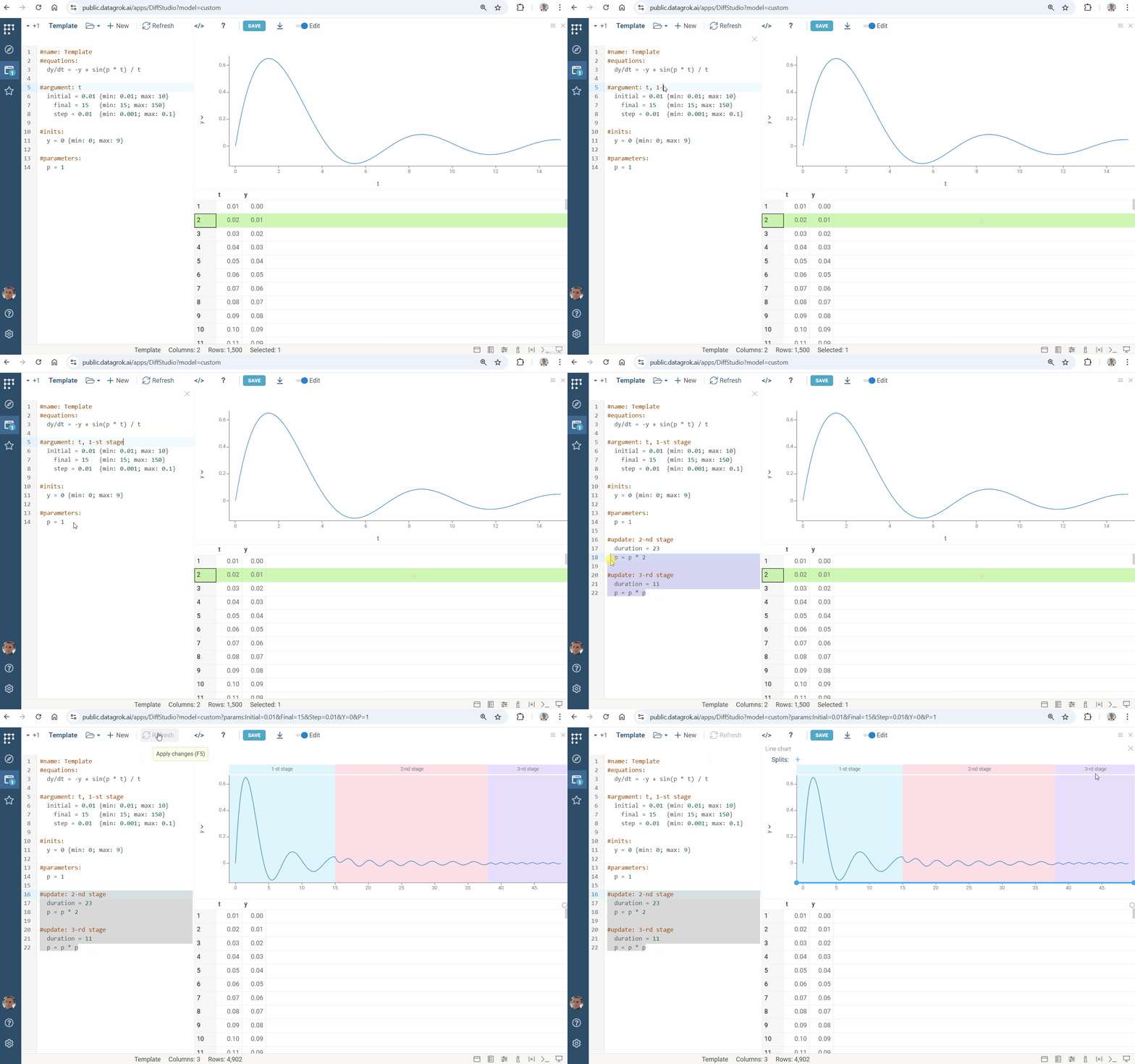
Use the #update block to construct models with multiple sequential processes (stages):
-
First stage is always defined in the
#argumentblock. Add the stage name:#argument: t, 1-st staget0 = 0.01t1 = 15h = 0.01 -
Subsequent stages are defined in the
#updateblocks. Specify:- Stage name
- Stage duration
- Parameter modifications. To define parameters, use any valid mathematical expression.
#update: 2-nd stageduration = 23p = p * 2
You can add any number of #update blocks to create simulation stages. Each stage appears in distinct color on the line chart:
User interface options
Diff Studio automatically generates the UI, but you can use the following options to improve usability:
-
Captions:
-
Define the desired captions for the input parameters. If no caption is provided, Diff Studio uses the variable name
#argument: tstart = 0 {caption: Initial time}finish = 2 {caption: Final time}step = 0.01 {caption: Calculation step} -
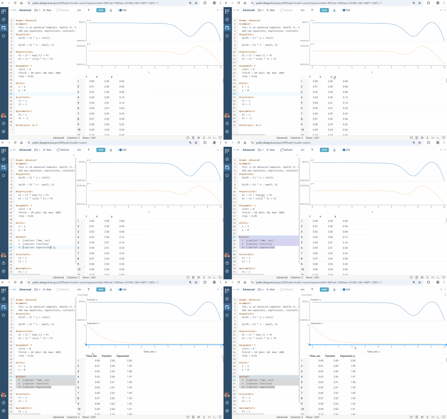
#output: Caption column headers in the solution table. If no caption is provided, Diff Studio uses the variable name#output:t {caption: Time, h}A1 {caption: Central}A2 {caption: Peripheral}Use this block to set any entity from
#equationsor#expressionsyou want included in the output:
-
-
Categories: Group related inputs together by specifying their category
#parameters:P1 = 1 {category: Parameters}P2 = -1 {category: Parameters} -
Units: Add measurement units
#inits:x = 2 {units: C; category: Initial values}y = 0 {units: C; category: Initial values} -
Tooltips: Provide tooltips in brackets
[ ]:P1 = 1 {category: Parameters} [P1 parameter tooltip] -
Input ranges: Set min/max values and step to create sliders and clickers for interactive model exploration
#inits:x = 2 {min: 0; max: 5}y = 0 {min: -2; max: 2; step: 0.1}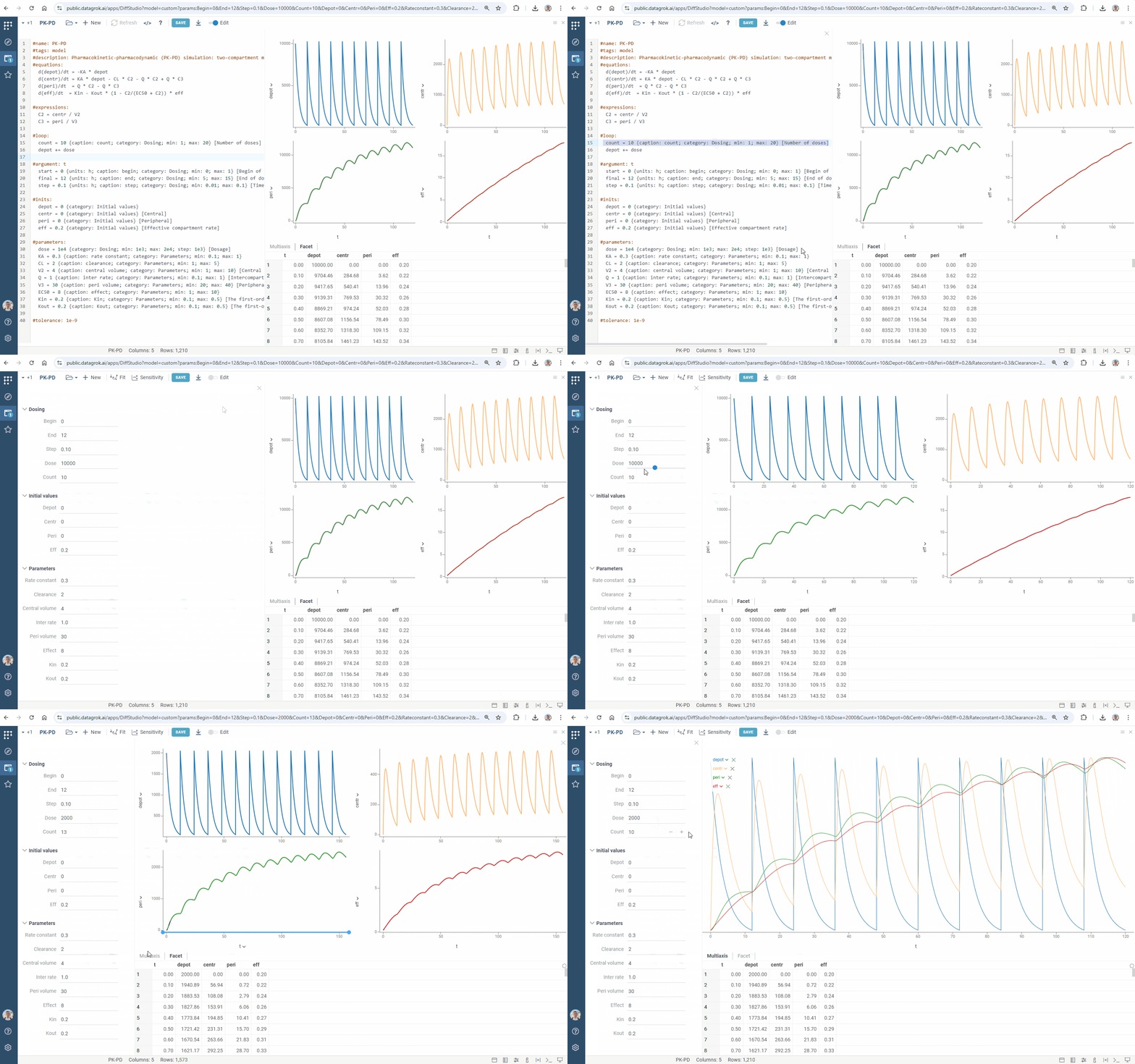
-
Lookup tables: The
#meta.inputsblock links model parameters to preset values in a lookup table. Upon linking, Diff Studio creates a dropdown menu to switch between parameter sets and automatically populates model inputs based on the selected preset. To add a lookup table:-
Create a CSV file with parameter sets and upload it to Datagrok
x y ... Set 1 1 2 ... Set 2 3 4 ... -
Link file to model using the
#meta.inputsblock. Optionally, add a caption, category, and a tooltip:
#meta.inputs: table {choices: OpenFile("System:AppData/DiffStudio/inputs.csv"); caption: [UI label]; category: [Group name]} [Tooltip]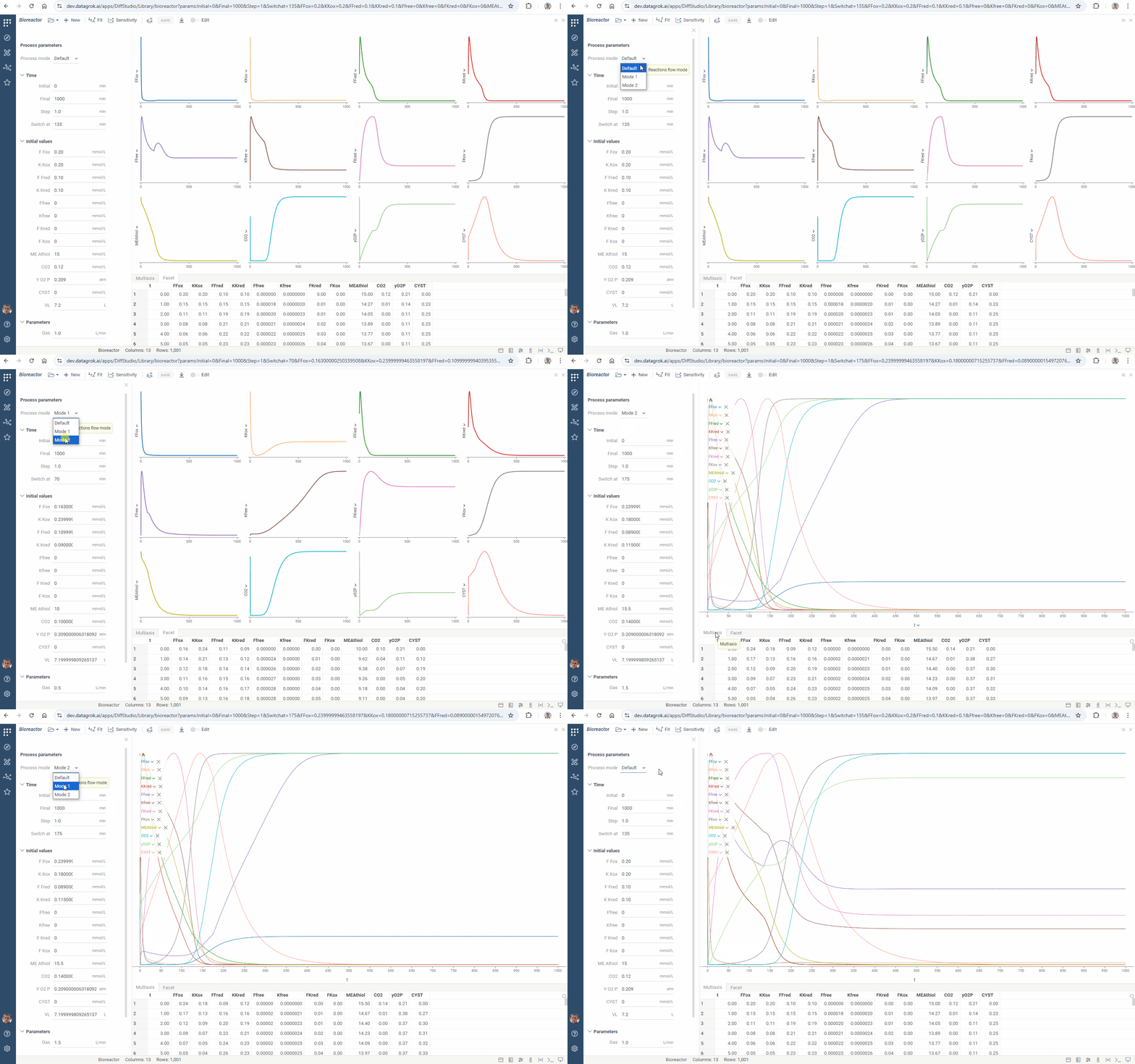
-
Solver configuration
Use this syntax to define the ODE solver configuration and improve performance:
-
#meta.solver: Defines numerical solver settings:- Method: Choose from the following solvers:
- Implicit methods (for stiff ODEs) - Rosenbrock-Wanner type:
- The ROS34PRw method (
ros34prw, default) - The ROS3PRw method (
ros3prw) - The modified Rosenbrock triple (
mrt)
- The ROS34PRw method (
- Explicit methods (for non-stiff ODEs):
- The Bogacki-Shampine 3(2) method (
rk3) - The Runge-Kutta-Fehlberg 4(5) method (
rk4) - The Dormand-Prince 5(4) method (
rkdp) - The Adams multistep predictor-correctors methods of order 4 and 5 (
ab4,ab5)
- The Bogacki-Shampine 3(2) method (
- Adaptive solvers:
- Implicit methods (for stiff ODEs) - Rosenbrock-Wanner type:
- Performance limits
maxTimeMs: computation time, in milliseconds (default: 5000ms)maxIterations: iteration count for debugging
#meta.solver: {method: 'mrt'; maxTimeMs: 50} - Method: Choose from the following solvers:
-
#tolerance: Defines numerical method precision#tolerance: 0.00005
Platform integration
You can convert Diff Studio models to Datagrok scripts. This allows you to:
- Add your models to a Model Hub.
- Access advanced platform features and create reusable components with rich UI (learn more).
Click the Save to Model Hub icon on the top panel to add your model to Model Hub:
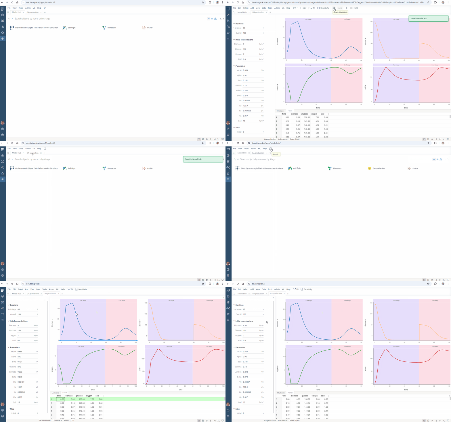
Export your model to JavaScript script:
-
Toggle Edit and click the
</>icon -
Add metadata for catalog:
//tags: model//description: Brief description -
Click SAVE. The script is created and can be found in Browse > Platform > Functions > Scripts. The conversion preserves all input annotations, maintaining intuitive UI controls.
Syntax reference
Diff Studio lets you define a model in a declarative form using simple syntax:
| Keyword | Specifies | Example |
|---|---|---|
| #name | Model name | Basic template, Robertson's model |
| #equations | Ordinary differential equations (ODEs) | Basic template, mass-action kinetics simulation |
| #inits | Initial conditions | Basic template, fermentation modeling |
| #argument | The independent variable, its range, and the solution time step | Basic template, pollution model |
| #expressions | Additional computations | Advanced template, pharmacokinetics simulation |
| #parameters | Model parameters (Diff Studio creates UI inputs for them) | Advanced template, chemical reactions modeling |
| #constants | Model constants | Advanced template, bioreactor model |
| #loop | Multiple simulation cycles | Pharmacokinetic-pharmacodynamic simulation |
| #update | Additional modeling stage | Gluconic acid production modeling |
| #output | Customized model output | Nimotuzumab disposition model |
| #tolerance | Tolerance of the numerical method | Advanced template, pollution model |
| #meta.inputs | CSV file with inputs lookup table | Bioreactor model |
| #meta.solver | ODEs solver settings | Pharmacokinetics simulation |
| #comment | Explanations, notes, remarks, etc. | Advanced template |
| #description | The platform script tooltip | Extended template |
To improve UI, annotate model inputs using:
| Option | Specifies | Example |
|---|---|---|
| caption | Input caption | Extended template |
| category | Input category. Items belonging to the same category are grouped together in the UI | Extended template |
| units | Input measure units | Mass-action kinetics simulation |
| min, max | Input min and max values, respectively. Use them to get sliders for UI input | Extended template |
See also
-
Videos:
