Multivariate analysis

Multivariate analysis (MVA) is based on the statistical principle of multivariate statistics, which involves observation and analysis of more than one statistical outcome variable at a time.

Partial least squares regression (PLS regression) is a particular type of MVA. PLS provides quantitative multivariate modelling methods, with inferential possibilities similar to multiple regression, t-tests and ANOVA. It constructs linear model using latent factors that

• maximally summarize the variation of the predictors
• maximize correlation with the response variable.

Regress and analyze

1. Open a table.
2. On the Top Menu, select ML | Analyze | Multivariate Analysis.... A dialog opens.
3. In the dialog, specify
   • the column with response variable (in the Predict field)
   • the columns with the predictors (in the Using field)
   • the number of Components, i.e. latent factors
   • Names of data samples
4. Press Run to execute. You get
   • the Observed vs. Predicted scatterplot comparing the response to its prediction
   • the Scores scatterplot reflecting data samples similarities and dissimilarities
   • the Loadings scatterplot indicating the impact of each feature on the latent factors
   • the Regression Coefficients bar chart presenting parameters of the obtained linear model
   • the Explained Variance bar chart measuring how well the latent factors fit source data

Observed vs. Predicted

The Observed vs. Predicted scatterplot compares the response variable to its prediction. The coefficient of determination r2 indicates the goodness of fit:

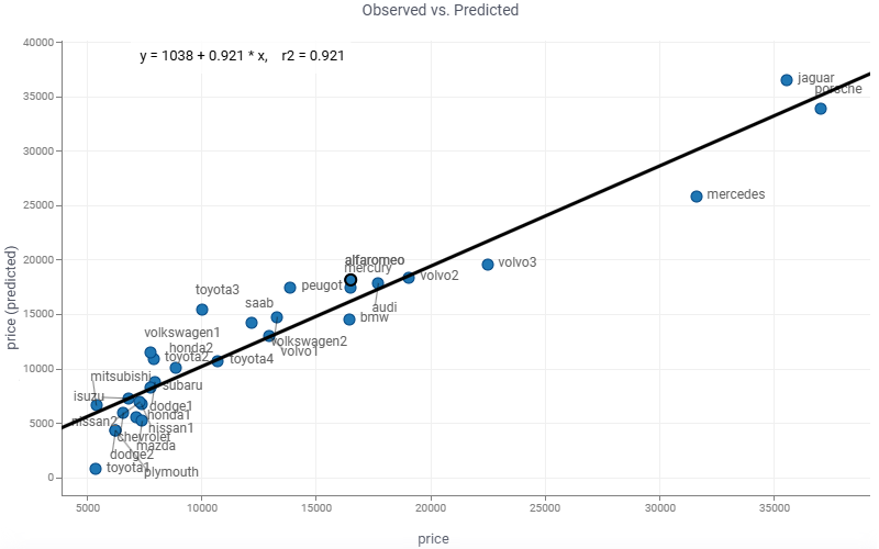
Combine it with the Scores scatterplot to explore data samples:

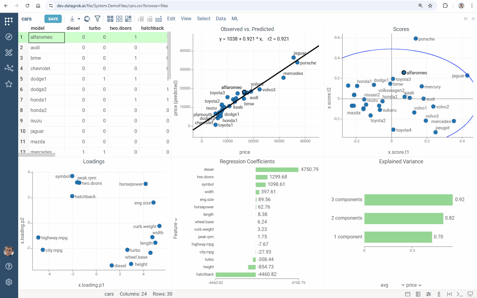
Scores

The Scores scatterplot shows the values of the latent factors for each observation in the dataset:

• the predictors (T-scores)
• the response variable (U-scores).

It indicates correlations between observations (how observations related to each other, occurrence groups or trends).

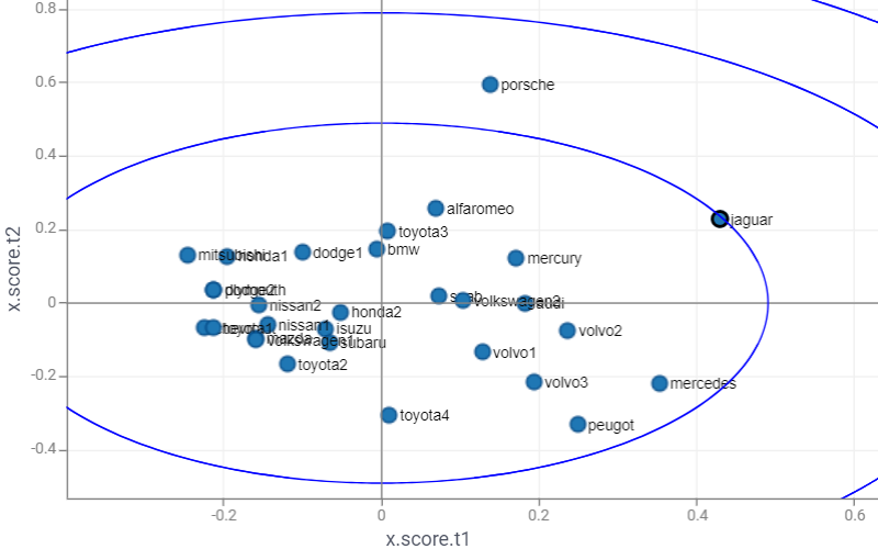
Combine it with the Observed vs. Predicted scatterplot to explore data samples:

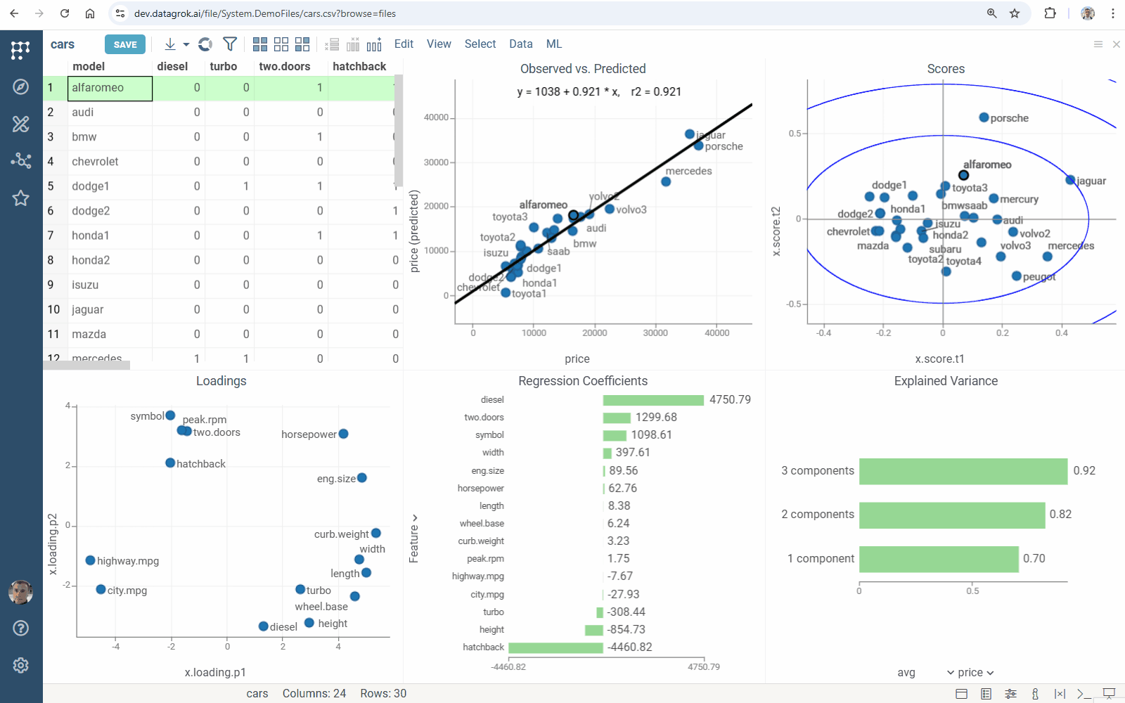
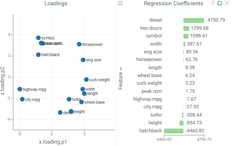
Loadings

The Loadings scatterplot visually represents the influence of each feature on the latent factors: high loadings indicate a strong influence.

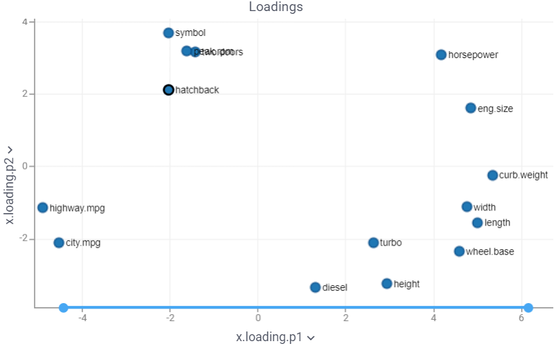
Use it in combination with the Regression Coefficients bar chart to explore features:

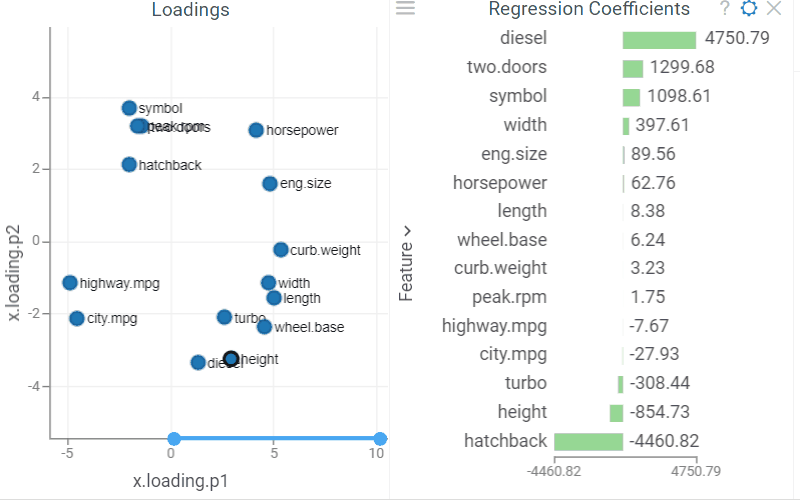
Regression coefficients

The Regression Coefficients bar chart presents parameters of the obtained linear model (used with the original data scale):

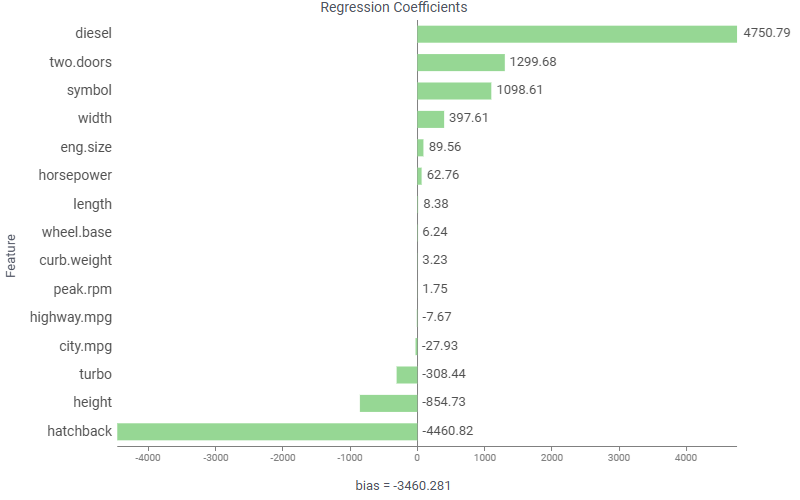
Combine it with the Loadings scatterplot to explore features:

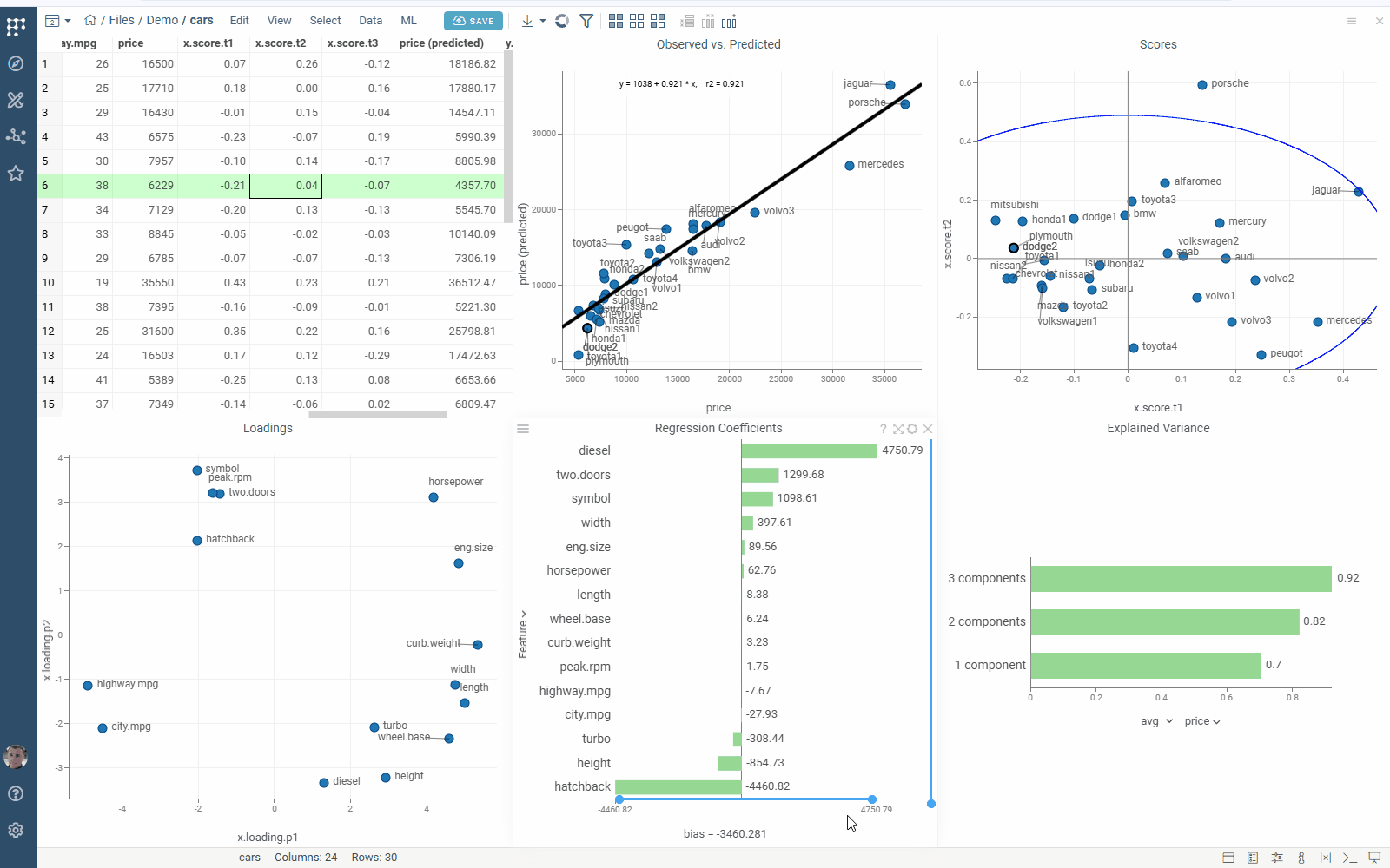
Explained variance

The Explained Variance bar chart shows the explained variance of variables by PLS-components, cumulative sum by each of components.

Use it to explore how well the latent components fit source data: closer to one means better fit.

PLS components

Compute the predictors representation by the latent factors:

1. Open a table.
2. On the Top Menu, select ML | Analyze | PLS.... A dialog opens.
3. In the dialog, specify
   • the column with response variable (in the Predict field)
   • the columns with the predictors (in the Using field)
   • the number of Components, i.e. latent factors

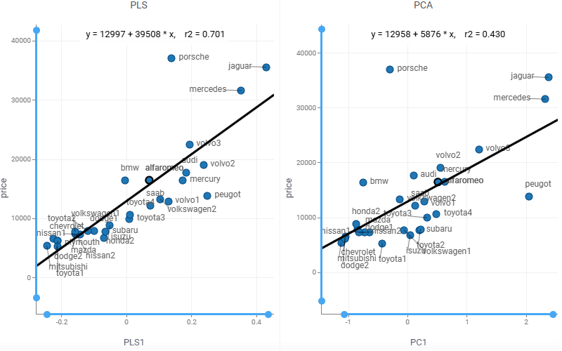
PLS components contain more predictive information than ones provided by principal component analysis (PCA). The coefficient of determination r2 indicates this:

See also

• Dimensionality reduction
• Analysis of variances
• Tutorial