Cheminformatics
Datagrok provides an intuitive, enterprise-ready high-performance environment for working with chemical data, covering full-range of tasks - from data access to de novo design.
- Data access
- Built-in connectors to 30+ data sources
- Automatic structure detection on import
- Support for SMILES, SMARTS, InChI, InChiKey, SDF, PDB, MOL2, and more
- Integration with compound registration systems
- Interactive exploration and analysis
- Highly customized 2D (RDKit or OpenChemLib) and 3D (NGL) rendering of molecules, rendering of chemical mixtures
- Powerful chemically-aware spreadsheet and viewers
- Chemical space and interactive structure search
- Comprehensive ML toolkit for clustering, dimensionality reduction, imputation, PCA/PLS, and more. Built-in statistics
- Dynamic dashboards
- Sketching and structure analysis
- Multiple molecular sketchers
- Tools for R-groups, scaffold trees, retrosynthesis, and elemental analysis
- SAR analysis
- Predictive and generative modeling
- QSAR/QSPR modeling and ADMET predictions
- Docking using AutoDock Vina
- Generative chemistry via REINVENT4
- Data augmentation and utilities
- Calculated columns using 500+ functions (or create your own)
- Chemical scripts and custom plugins
- Calculators, curation, mutation, virtual synthesis
To get started, install the required packages (see instructions).
Data access
Datagrok provides a single, unified access point for organizations. You can connect to any of the 30+ supported data sources, retrieve data, and securely share data with others.
Chemical queries against data sources require a chemical cartridge, such as RDKit Postgres cartridge or JChem cartridge. These cartridges allow molecule-specific operations (like substructure or similarity searches) to be integrated into SQL queries using SQL syntax.
Example: Substructure search in a database
To create a chemically-aware query, use the SQL syntax specific to your cartridge. Annotate parameters like you would for a function. Here is an example of querying ChEMBL on Postgres with the RDKit cartridge installed:
Substructure search:
--name: @pattern substructure search
--connection: chembl
--input: string pattern {semType: Substructure}
--input: int maxRows = 1000
 select molregno,m as smiles from rdk.mols where m@>@pattern
 limit @maxRows
Similarity search:
--name: @pattern similarity search
--connection: chembl
--input: string pattern {semType: Substructure}
--input: int maxRows = 1000
select fps.molregno, cs.canonical_smiles as smiles
from rdk.fps fps
join compound_structures cs on cs.molregno = fps.molregno
where mfp2%morganbv_fp(@pattern)
limit @maxRows
To run a query, sketch the substructure and click OK. Datagrok retrieves the data and opens it in a spreadsheet.

To learn more about querying data and data access in general, see the Access section of our documentation.
Compound registration systems
Datagrok integrates with compound registration systems. You can browse and analyze your assay data directly in the platform.
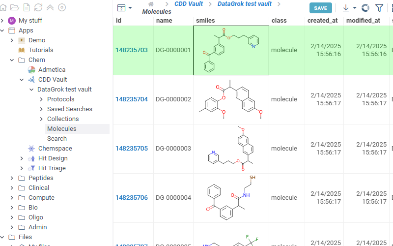
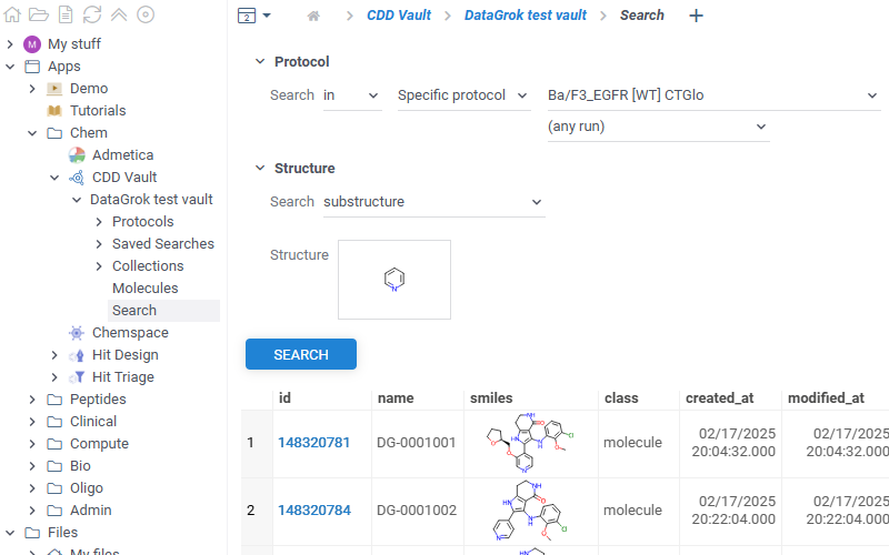
CDD Vault
Datagrok integrates with CDD Vault. You can:
- browse molecules available in the selected vault
- search vaults by similarity and substructure
- save searches and explore them in Datagrok
- view linked assay data for a target compound in the Context Panel
How to use
To use the app, you need to be registered in the CDD Vault system and have at least one vault set up.
The CDD Vault api key should be set in package credentials manager under apiKey key.
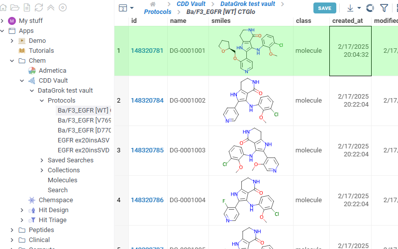
To access assay data, in the Browse panel, go to Apps > Chem > CDD Vault. The app lists all connected vaults. Each vault contains 3 sections. You can also explore the vault data directly in the Context Panel (Databases > CDD Vault). Watch a video tutorial (~2 mins).
- Molecules
- Protocols
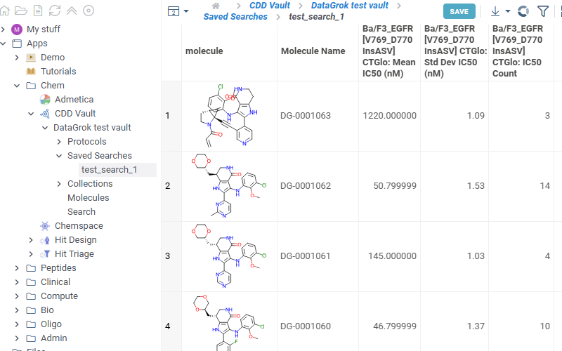
- Saved searches
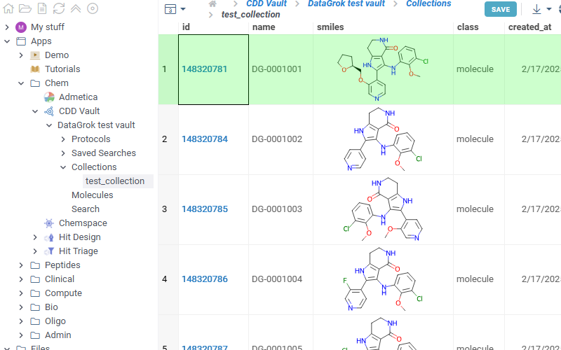
- Collections
- Search
- Context Panel
- Shows all molecules available in the selected vault
- The Id column contains contains direct links to corresponding molecules in your vault
- Shows all protocols available in the selected vault. Click any protocol to show corresponding molecules
Lists all saved searches in your vault. Click any search in the list to view its results
Lists all collections available in the selected vault. Click any collection to show corresponding molecules
Provides basic vault search functionality with similarity and diversity searches
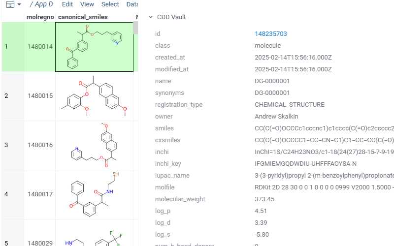
Shows vault data for the current molecule
Exploring chemical data
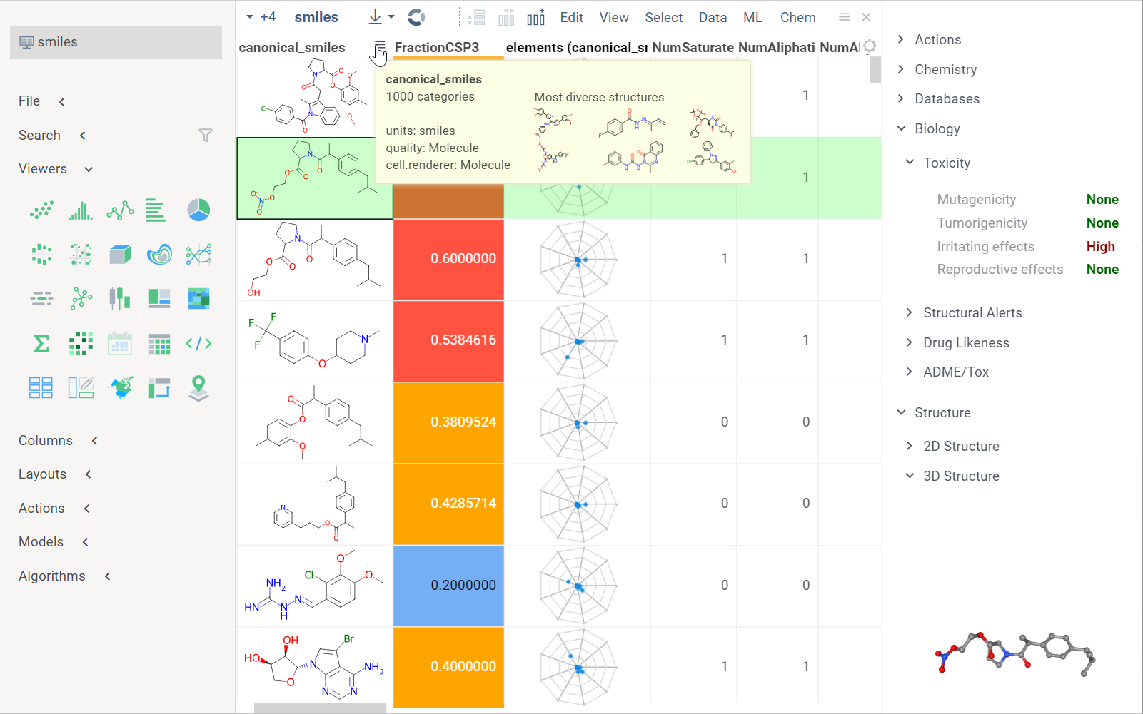
When you open a dataset, Datagrok automatically detects molecules and makes available molecule-specific context actions. For example, when you open a CSV file containing molecules in the SMILES format, the following happens:
- Data is parsed, and the semantic type molecule is assigned to the corresponding column.
- Molecules are automatically rendered in the spreadsheet.
- Column tooltip now shows the most diverse molecules in your dataset.
- Default column filter is now a sketcher-driven substructure search.
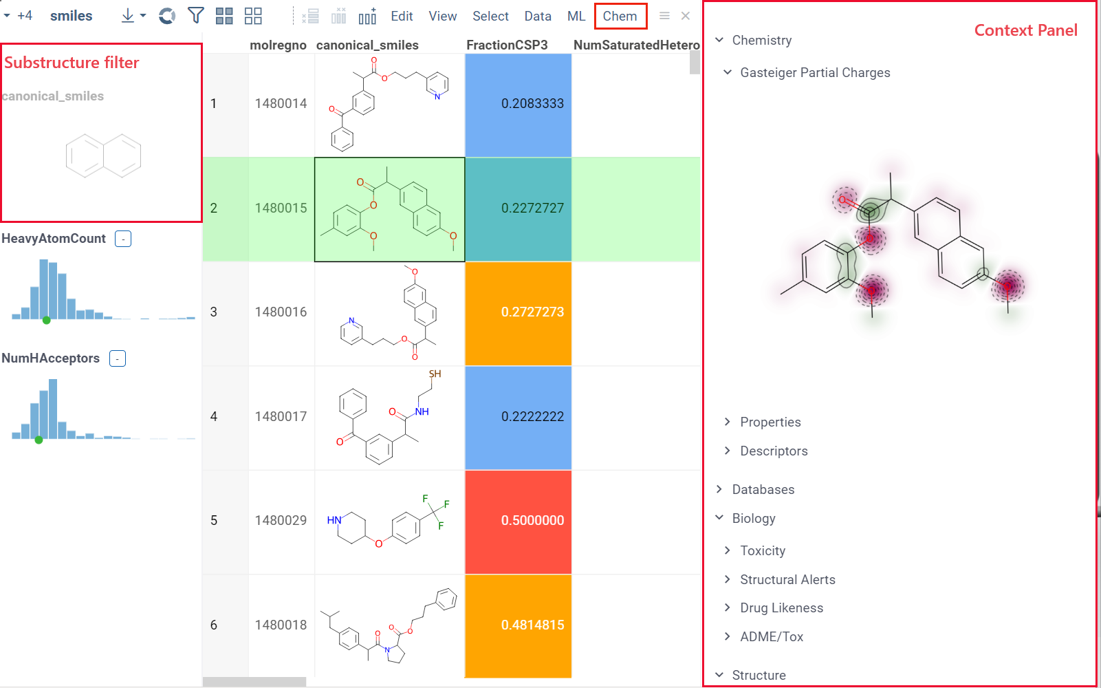
- A top menu item labeled Chem appears.
- When you click a molecule, the Context Panel on the right shows molecule-specific info panes, such as Toxicity or Drug Likeness (see the full list).
The following info panes are shown by default for the current molecular column:
- Most Diverse Structures
- Rendering (offers rendering options for molecules):
- Render a molecule or show its textual representation (Show structures).
- Aligned to a particular scaffold (Scaffold).
- Aligned to a scaffold defined in the specified column (Scaffold column).
- Highlight the scaffold (Highlight from column).
- Force regeneration for atom coordinates, even if the molecule is defined as a MOLBLOCK (Regenerate coords).
- Type of the filter for that column (sketcher or categorical)(Filter type).
Info pane options
Some info panes can customized. To reveal an info pane's available options, hover over it:
- View and/or edit the underlying script (click the Script icon).
- Change parameters (click the Parameter icon).
- Change the info pane's settings (click the Gear icon).
- Append info pane as a column (click the More actions icon and select Add as a column).
To learn how to customize and extend the platform programmatically, see the Develop section of our documentation.
Info panes can be extended with functions in any supported language.
Also Datagrok is capable of detecting and rendering mixtures. Mixtures should be in a Mixfile format introduced by Collaborative Drug Discovery, Inc. Mixfiles are automatically detected by Datagrok and the data is assigned with ChemicalMixture semantic type, allowing you to render mixtures of any complexity and retrieve detailed information through context panel. The main features are:
-
rendering of the list of components in one cell with clear differentiation between components (square brackets are used for nested mixtures). In case component quantity/ratio is present in the Mixfile, it is also shown within the cell
-
interaction with each mixture component straight from the grid cell. Hover over any component to get more details in the tooltip. Click on separate component to get structure details in the context panel
- summary of mixture information in the context panel. You can browse the mixture using either table or tree view
Chemically aware spreadsheet
The spreadsheet lets you visualize, edit, and efficiently work with chemical structures. Additionally, you can add new columns with calculated values or visualizations from info panes or context actions. The features also include the ability to interactively filter rows, color-code columns, pin rows or columns, set edit permissions, and more. To learn how to work with the spreadsheet, see this article or complete this tutorial.
Chemically aware viewers
Datagrok viewers recognize and display chemical data. The viewers were built from scratch to take advantage of Datagrok's in-memory database, enabling seamless access to the same data across all viewers. They also share a consistent design and usage patterns. Any action taken on one viewer, such as hovering, selecting, or filtering, is automatically applied to all other viewers, creating an interconnected system ideal for exploratory data analysis.
In addition to the chemical spreadsheet, examples of viewers include a scatterplot, a network diagram, a tile viewer,a bar chart, a form viewer, and trellis plot, and others. All viewers can be saved as part of the layout or a dashboard. Some viewers offer built-in statistics.
To learn how to use viewers to explore chemical data, complete this tutorial or visit the Visualize section of our documentation.
You can add custom viewers.
Chemical space
Analyze chemical space using distance-based dimensionality reduction algorithms, such as tSNE and UMAP. These algorithms use fingerprints to convert cross-similarities into 2D coordinates. This allows to visualize the similarities between molecular structures and identify clusters of similar molecules, outliers, or patterns that might be difficult to detect otherwise. The results are visualized on the interactive scatterplot.
How to use
Go to the Top Menu Ribbon and choose Chem > Analyze > Chemical Space... This opens a Chemical Space parameter dialog.
The dialog has the following inputs:
-
Table: The table containing the column of sequences.
-
Column: The column containing the sequences.
-
Encoding function: The encoding function that will be used for pre-processing of molecules. Currently, only one encoding function is available, that will use chemical fingerprint distances between each molecule to calculate pairwise distances. The
Fingerprintsfunction has 1 parameter which you can adjust using the gear (⚙️) button next to the encoding function selection:- Fingerprint type: The type of molecular fingerprints that will be used to generate monomer substitution matrix. Options are
Morgan,PatternorRDKit.
- Fingerprint type: The type of molecular fingerprints that will be used to generate monomer substitution matrix. Options are
-
Method: The dimensionality reduction method that will be used. The options are:
-
UMAP: UMAP is a dimensionality reduction technique that can be used for visualization similarly to t-SNE, but also for general non-linear dimension reduction.
- t-SNE: t-SNE is a machine learning algorithm for dimensionality reduction developed by Geoffrey Hinton and Laurens van der Maaten. It is a nonlinear dimensionality reduction technique that is particularly well-suited for embedding high-dimensional data into a space of two or three dimensions, which can then be visualized in a scatterplot.
Other parameters for dimensionality reduction method can be accessed through the gear (⚙️) button next to the method selection.
-
-
Similarity: The similarity/distance function that will be used to calculate pairwise distances between fingerprints of the molecules. The options are:
Tanimoto,Asymetric,CosineandSokal. All this distance functions are based on the bit array representation of the fingerprints. -
Plot embeddings: If checked, the plot of the embeddings will be shown after the calculation is finished.
-
Postprocessing: The postprocessing function that will be applied to the resulting embeddings. The options are:
- None: No postprocessing will be applied.
- DBSCAN: The DBSCAN algorithm groups together points that are closely packed together (points with many nearby neighbors), marking as outliers points that lie alone in low-density regions (whose nearest neighbors are too far away). The DBSCAN algorithm has two parameters that you can adjust through the gear (⚙️) button next to the postprocessing selection:
- Epsilon: The maximum distance between two points for them to be considered as in the same neighborhood.
- Minimum points: The number of samples (or total weight) in a neighborhood for a point to be considered as a core point. This includes the point itself.
- Radial Coloring: The radial coloring function will color the points based on their distance from the center of the plot. The color will be calculated as a gradient from the center to the border of the plot.
WebGPU (experimental)
WebGPU is an experimental feature that allows you to use the GPU for calculations in browser. We have implemented the KNN graph generation (with support to all simple and non-trivial distance functions like Tanimoto, Cosine, etc.) and UMAP algorithms in webGPU, which can be enabled in the dimensionality reduction dialog. This can speed up the calculations significantly, especially for large datasets, up to 100x. This option can be found in the gear (⚙️) button next to the method selection (UMAP).
Please note, that webGPU is still considered as experimental feature, and for now only works in Chrome or Edge browsers (although it is planned to be supported in Firefox and Safari in the future). If webGPU is not supported in your browser, this checkbox will not appear in the dialog. To make sure that your operating system gives browser access to correct(faster) GPU, you can check the following:
- Go to settings and find display settings
- Go to Graphics settings.
- In the list of apps, make sure that your browser is set to use high performance GPU.
Sketching
Datagrok provides integrations with various sketchers, but their availability depends on their licensing options. Some sketchers require a commercial license from the vendor before they can be used in Datagrok. To use these sketchers, you must provide a path to the license server.
How to provide a license path
- Go to Manage > Packages and select a package that you want to use.
- Navigate to the Context Panel > Settings and enter the license path in the License path field.
- Click SAVE to activate the license.
To launch a sketcher, double-click a molecule. Alternatively, in the Actions info pane, select Sketch.
You can sketch a molecule or retrieve one by entering SMILES, compound identifier, or a common name (like aspirin). The following compound identifiers are natively understood since they have a prefix that uniquely identifies the data source: SMILES, InChI, InChIKey, ChEMBL, MCULE, comptox, and zinc (example: CHEMBL358225). The rest of the 30+ identifier systems can be referenced by prefixing the source name followed by a colon to the identifier (example: 'pubchem:11122').
Supported identifier systems
| actor | drugbank | lipidmaps | pubchem |
| atlas | drugcentral | mcule | pubchem_dotf |
| bindingdb | emolecules | metabolights | pubchem_tpharma |
| brenda | fdasrs | molport | recon |
| carotenoiddb | gtopdb | nih_ncc | rhea |
| chebi | hmdb | nikkaji | selleck |
| chembl | ibm | nmrshiftdb2 | surechembl |
| chemicalbook | kegg_ligand | pdb | zinc |
| comptox | lincs | pharmgkb |
You can register a function to instruct Datagrok to retrieve molecules from a database using custom identifiers. To do so, annotate the function with the following parameters: --meta.role: converterand --meta.inputRegexp:. These annotations provide the necessary instructions for Datagrok to recognize the function as a converter and handle the input appropriately.
Example
The following code snippet defines a converter function that retrieves the SMILES representation of a molecule from the ChEMBL database using the provided ChEMBL identifier. The output is the canonical SMILES string representing the molecule.
--name: chemblIdToSmiles
--friendlyName: Converters | ChEMBL to SMILES
--meta.role: converter
--meta.inputRegexp: (CHEMBL[0-9]+)
--connection: Chembl
--input: string id = "CHEMBL1185"
--output: string smiles { semType: Molecule }
--tags: unit-test
select canonical_smiles from compound_structures s
join molecule_dictionary d on s.molregno = d.molregno
where d.chembl_id = @id
--end
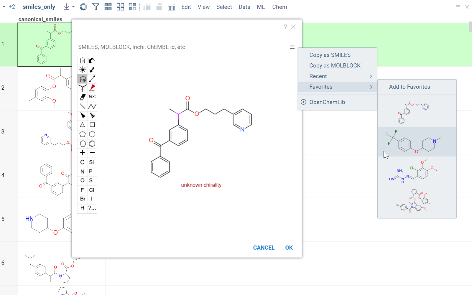
From the Hamburger (☰) menu, you can access the following features:
- Copy a molecule as SMILES or MOLBLOCK.
- View recently sketched structures.
- View/add to favorites.
- Switch between available sketchers. Datagrok remembers your preferred sketcher type, so you don't have to select it every time you use it.
Sketchers are synchronized with the Context Panel. As you draw or edit a molecule, the info panes on the right dynamically update with the information about the sketched compound.
Structure search
Substructure search / Filtering
Datagrok offers an intuitive filtering functionality to explore and filter datasets. Hovering over categories or distributions in the Filter Panel instantly highlights relevant data points across all viewers. For molecules, Datagrok uses integrated sketchers to allow structure-based filtering. After applying the filter, Datagrok highlights the queried substructures in the filtered subset.
How to use
To filter by substructure, follow these steps:
- On the Menu Ribbon, click the Filter icon to open the Filter Panel. The panel shows filters for all dataset columns. By default, the substructure filter is displayed on top, but you can rearrange, add, or remove filter columns by using available controls.
- Open the sketcher by clicking the Click to edit button. Sketch or enter a substructure.
- Once finished, click OK to apply the filter.
To clear the filter, use the checkbox provided. To remove the filter altogether, use the Close (x) icon.
To learn more about filtering, watch this video or read this article.
Similarity and diversity search
Datagrok offers two analytical tools to help you analyze a collection of molecules based on molecular similarity: similarity search and diversity search. Similarity search finds structures similar to the reference molecule, while diversity search shows N molecules of different chemical classes presented in the dataset. Both tools are based on fingerprints, with the customizable distance metric.
Available distance metrics
- Tanimoto
- Dice
- Cosine
To sort a dataset by similarity, right-click your reference molecule and select Current value > Sort by similarity. The dataset is sorted with the reference molecule pinned at the top.
To explore the dataset further, use the similarity and diversity viewers (Top Menu > Chem > Search > Similarity Search... or Diversity Search...). The viewers are interactive and let you quickly switch between the molecules of interest.
How to use
To configure a similarity or diversity viewer, click the Gear icon at the viewer's top. The Context Panel updates with available controls. You can change parameters like the similarity threshold, fingerprint type, or the distance measure.
By default, a reference molecule follows the current row. If you click a different molecule, the similarity viewer updates accordingly. To lock in a specific reference molecule, clear the Follow Current Row control. To sketch a custom reference molecule, click the Edit icon on the reference molecule card.
You can enhance the viewer cards by incorporating column data. To do so, use the Molecule Properties control. If a column is color-coded, its format is reflected on the card's value. To adjust how the color is shown (either as a background or text), use the Apply Color To control. To remove highlighting, clear the color-coding from the corresponding column in the dataset.
External data sources
Datagrok integrates with multiple data sources to enable structure-based search, including:
- ChEMBL
- DrugBank
- PubChem (supports identity search)
- SureChEMBL (search patented molecules similar to your compounds)
- Chemspace (includes filters by shipping country and compound category)
To see the full list, see Plugins.
To run a substructure or similarity search, either sketch or click a molecule in your dataset and expand the Databases section of the Context Panel to view matches for your target molecule. You can also open the results in a separate Table View by clicking the plus (+) icon within the relevant info pane.
To dynamically enrich compound IDs with linked data,
register identifier patterns
(e.g., CHEMBL\d+). Once registered, the matching values:
- are automatically detected and highlighted across the platform
- show linked content on click, hover, and in search results
This is especially useful when working with diverse identifiers from sources like GDB exports, internal registries, or assay results.
Structure analysis
R-groups analysis
R-group analysis decomposes a set of molecules into a core and R-groups (ligands at certain attachment positions), and visualizes the results. The query molecule consists of the scaffold and ligand attachment points represented by R-groups. R-group analysis runs in browser using RDKit JS library.
How to use
- Workflow
- Only match at R groups
- Go to Chem > Analyze > R-Groups Analysis... A sketcher opens.
- In the sketcher, specify the common core (scaffold) for the selected molecular column using one of these methods:
- Draw or paste a scaffold in the sketcher. You can define core with custom enumerated R groups.
- Click MCS to automatically identify the most common substructure.
- Click the Gear icon to adjust R group analysis parameters.
- Click OK to execute. The R-group columns are added to the dataframe, along with a trellis plot for visual exploration.
R-groups are highlighted with different colors in the initial molecules in grid. Molecules are automatically aligned by core. To filter molecules with R group present in each enumerated position use isMatch column.
The trellis plot initially displays pie charts. To change the chart type, use the Viewer control in the top-left corner to select a different viewer.
If you prefer not to use a trellis plot, close it or clear the Visual analysis checkbox during Step 3. You can manually add it later. You can also use other chemical viewers, like scatterplot, box plot, bar chart, and others.
Use Replace latest checkbox to remove previous analysis results when running the new one. Or check it to add new analysis results in addition to existing.
You can restrict R-groups analysis to molecules that have actual substituents at the specified R-group positions:
- Define a core with labeled R-groups in the sketcher
- Click the Gear icon and enable Only match at R groups. Before running the analysis, the tool verifies that the core contains properly labeled R groups. The selected setting is saved automatically for future sessions.
To run the r-group decomposition programmatically, see this sample script.
Scaffold tree analysis
The scaffold tree viewer viewer organizes molecules into a hierarchical tree based on their scaffolds, making it easy to explore structure-activity relationships, filter datasets, and navigate chemical space.
You can:
- Automatically generate scaffold trees using a customized ScaffoldGraph algorithm
- Manually sketch the tree or edit nodes
- Highlight matching molecules, filter datasets, and color-code scaffolds for easy profiling
The scaffold tree is synchronized with other viewers and can be saved as part of a layout or dashboard.
How to use
- Anatomy
- Add
- Edit
- Selection and filtering
- Color-code
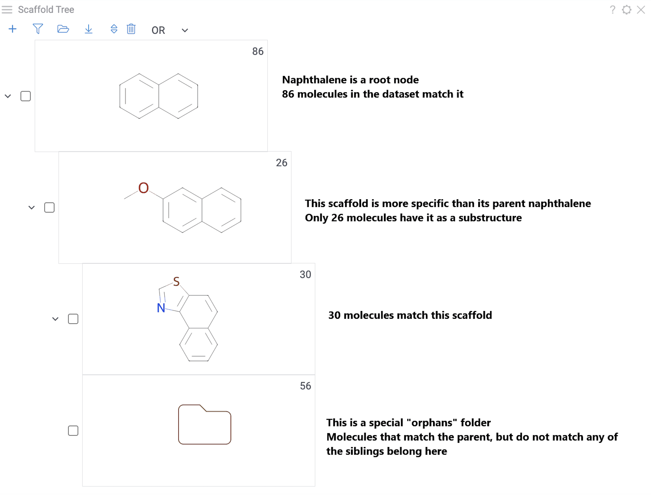
Each node represents a scaffold. Nodes form a hierarchy where:
- The root scaffold is the smallest common substructure
- Child scaffolds contain their parent as a substructure
- Each scaffold builds on the structure above it in the tree
- Orphan nodes contains the parent scaffold but don't have any sibling scaffolds
Generate automatically:
- Go to Top Menu > Chem > Analyze > Scaffold Tree. This adds the scaffold tree viewer to your dataset.
- On the viewer, click Generate to build the tree. Generation may take several minutes for large datasets.
Load from your computer:
- To download, click the Download icon at the top of the viewer.
- To upload, click the Open icon at the top of the viewer and select your file.
Sketch manually:
- Go to Top Menu > Chem > Analyze > Scaffold Tree. This adds the viewer to your dataset.
- To create the root scaffold, at the top of the viewer, click the Add new root structure (+) icon and sketch your structure.
- To add scaffolds below, click the Add new scaffold (+) icon on a scaffold and sketch.
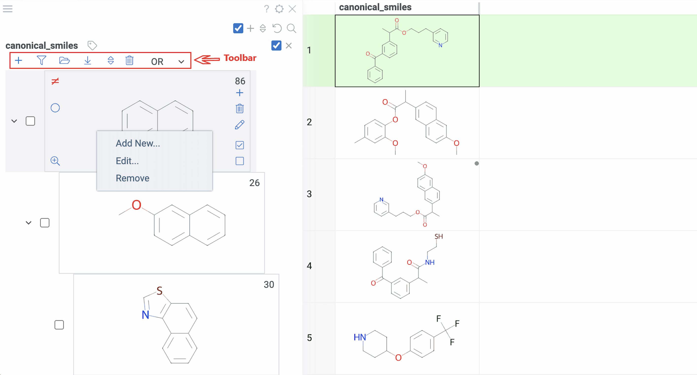
Tip: The viewer's toolbar icons appear when the viewer is active or when you hover over it.
Viewer controls (top of viewer):
- Clear all scaffolds: Click the Drop all trees (trash) icon
- Add root scaffold: Click the Add new root structure (+) icon
Scaffold controls (on each scaffold card):
- Add scaffold below: Click the Add new scaffold (+) icon
- Edit scaffold: Click the Edit icon to sketch
- Delete scaffold: Click the Remove scaffold (trash) icon to delete the scaffold and all scaffolds below it
Tip: You can also right-click any scaffold for these options: Add New..., Edit..., or Remove.
Selection:
- Highlight rows: Hover over any scaffold
- Select rows: Click the Select rows icon on the scaffold
- Deselect rows: Click the Deselect rows icon on the scaffold
- Exclude from selection: Click the ≠ icon on the scaffold (inverts the selection state)
Filtering:
- Filter by scaffold: Click it
- Exclude from filtered subset: Click the ≠ icon on the scaffold (inverts the filtered state)
- Clear filters: At the top of the viewer, click the Filter icon.
To select or filter by multiple scaffolds, select the checkbox to the left of each desired scaffold. Use the AND/OR control at the top of the viewer to define the logic:
- OR (default): includes rows matching any selected scaffold
- AND: includes only rows matching all selected scaffolds
Selections and filters sync across all viewers in your dataset. You can use the scaffold tree in combination with other filters.
Color scaffolds to highlight relationships. The colors appear both in the dataset column and the scaffold tree.
- To toggle coloring, on the scaffold, click the Circle icon. When off, the node inherits color from its nearest colored parent.
- To assign new color, click the Palette icon. The color applies to the scaffold and all its child scaffolds unless they already have custom colors.
- To override an inherited color, assign the new color. Custom node colors takes precedence.
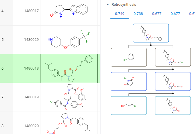
Retrosynthesis
You can explore the most efficient synthetic pathways and commercially available starting materials for your target molecules. To view the results for your target, click or sketch a molecule, and expand the Retrosynthesis pane in the Context Panel. Requires the Retrosynthesis plugin.
How to use
Watch a video tutorial (~3 mins).
To explore retrosynthesis pathways for a compound:
- Select a target molecule: Click on a molecule in your dataset or sketch one
- In the Context Panel, open the Retrosynthesis pane
- View routes: Each tab shows a different pathway, ranked by score based on stock availability, route length, and confidence. The best routes appear first
- Interact with the results:
- Click any precursor or intermediate to view its details in the Context Panel
- Hover over a pathway to reveal action icons, then click the Add to workspace (+) icon to open the entire pathway in a separate Table View
You can use custom models, stock databases, and display parameters (e.g., route length).
To set up a custom configuration:
-
Create a configuration folder: Go to Browse > AppData > Retrosynthesis > configs and create a folder with your custom configuration name
-
Add required files to your configuration folder. The minimum required files are:
- Expansion model
- Templates file
- Stock file
config.ymlwith file paths and parameters
-
Define file paths in
config.yml. Paths must follow this format:/app/aizynthcli_data/configs/<your_custom_config_name>/<file_name>IMPORTANT: Correct path naming is critical for the configuration to work properly.
Example:
 expansion:
   full:
     - /app/aizynthcli_data/configs/my_config/my_expansion_model.onnx
     - /app/aizynthcli_data/configs/my_config/my_templates.csv.gz
 stock:
my_stock: /app/aizynthcli_data/configs/my_config/my_stock.hdf5 -
Apply your configuration: Hover over any route and click the gear icon, and select your custom configuration as the current one.
Elemental analysis
Elemental Analysis analyzes the elemental composition of a molecular structure and visualizes the results in a radar viewer. Each point on the chart represents an element, and the distance from the center of the chart to the point indicates the relative abundance of that element in the structure. Use it as a basic tool to explore the dataset and detect rare elements and unique properties.
How to use
- In the Menu Ribbon, open the Chem menu and select Analyze structure > Elemental Analysis... A parameter input dialog opens.
- In the dialog:
- Select the source table and the molecular column that you want to analyze.
- Select the desired visualization option. You can choose between a standalone viewer (select Radar View) and sparklines (select Radar Grid), both of which use a radar viewer.
- Click OK to execute the analysis. New columns with atom counts and molecule charges are added to the spreadsheet and plotted on a radar chart using the selected visualization option.
Structure relationship analysis
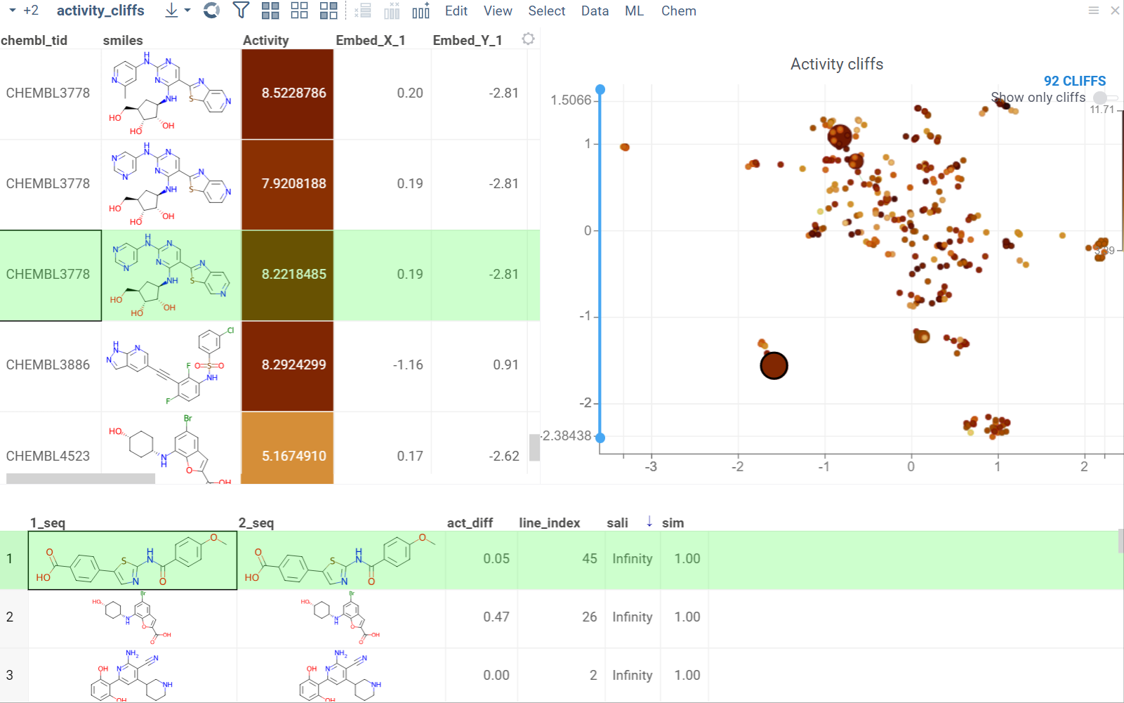
Activity cliffs
The Activity Cliffs tool in Datagrok detects and visualizes pairs of molecules with highly similar structures but significantly different activity levels, known as "activity cliffs." This tool uses distance-based dimensionality reduction algorithms (such as tSNE and UMAP) to convert cross-similarities into a 2D scatterplot.
How to use
- Open the Chem menu and select Analyze SAR > Activity Cliffs.
- In the parameter input dialog, specify the following:
- Select the source table, molecular column, and activity data column to analyze.
- Set the similarity cutoff.
- Select a dimensionality reduction algorithm and adjust its parameters using the Gear icon next to the Method control.
- Click OK to execute the analysis. A scatterplot visualization is added to the view.
- Optional. In the scatterplot, click the link with the detected number of cliffs to open an Activity Cliffs table containing all pairs of molecules identified as cliffs. The tables also have detailed information such as similarity score, activity difference score, and other data.
In the scatterplot, the marker color corresponds to the level of molecule activity, and the size represents the maximum detected activity cliff for that molecule. The opacity of the line connecting molecule pairs corresponds to the size of the activity cliff.
To explore the molecule pairs:
- Click a molecule in the source dataframe to zoom in on the scatterplot and focus on the pair that includes the selected molecule. Hover over molecule pairs and connecting lines to see summary information about them.
- Click the line connecting molecules in the scatterplot to select a corresponding pair of molecules in the underlying dataframe and Activity Cliffs table. The reverse also applies: clicking a pair in the Activity Cliffs table updates the scatterplot and selects the corresponding rows in the underlying dataframe.
As you browse the dataset, the Context Panel updates with relevant information.
Matched molecular pairs
The Matched Molecular Pairs (MMP) tool supports lead optimization by quantifying how specific structural changes affect potency, solubility, permeability, and ADMET properties across your dataset.
MMP analysis automatically detects matched molecular pairs within your dataset, calculates the differences in their properties, and aggregates these results. The mean property change derived from these transformations highlights consistent structure-activity relationships, indicating the expected effect of applying a similar modification to a new molecule.
The results of the MMP analysis are presented in a series of tables and visualizations, allowing you to:
- Identify high-impact structural modifications that enhance target properties
- Evaluate how specific chemical changes affect a compound's profile
- Generate optimized molecules with predicted properties based on transformations data
How to use
To run MMP analysis:
- In the Top Menu, select Chem > Analyze > Matched Molecular Pairs... to open the analysis dialog.
- In the dialog, configure the analysis by selecting:
- Table: The dataset you want to analyze
- Molecules: The column containing molecules
- Activities: One or more numerical columns representing activity or
property values. For each activity, you can set:
- Difference type: delta (x − y) or ratio (x / y)
- Scaling: none, log10, or −log10 (log options are available only when all values are non-negative)
- Cutoff: The maximum allowed fragment size relative to the core (default 0.4)
- Click OK. An MMP analysis is added to the view with four tabs:
When you first open the analysis, interactive hints guide you through the key features on each tab. Click Next to advance or Do not show to dismiss hints permanently.
- Substitutions
- Fragments
- Cliffs
- Generation
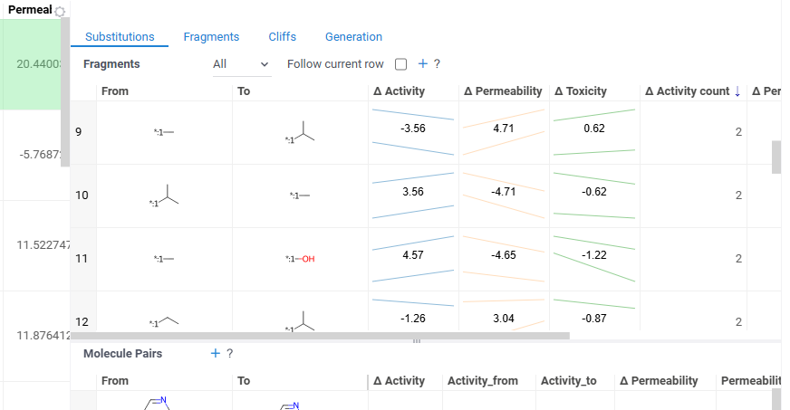
The Substitutions tab has two interactive tables:
-
Fragments table (upper): Shows all fragment substitutions found in your dataset along with their frequency, mean change in activity, and pair counts per activity. Mean activity columns use a compact in-cell visualization: each cell displays the mean difference value overlaid on a set of lines connecting individual "from" and "to" activity values for every pair in the substitution, giving you an at-a-glance view of both the trend and the spread.
It has two viewing modes:
- All: Shows all fragment pairs. Clicking a row highlights molecules in your dataset that contain either fragment from the current substitution.
- Current molecule: Shows only fragment pairs relevant to the currently selected molecule in your dataset, enabling exploration of molecule-specific substitutions.
Use the Follow current row toggle to automatically filter the Molecule pairs table based on the currently selected fragment pair.
Clicking a mean activity cell in the Fragments table opens a parallel coordinates plot in the Context Panel, showing individual activity values for all molecule pairs with that substitution.
-
Molecule pairs table (lower): Shows pairs of molecules and their property changes corresponding to the current substitution in the Fragments table. Clicking a row pins the molecule pair at the top of your dataset and shows the pair's details in the Context Panel, including all properties from the source table with substructure highlighting of the changed fragments.
To select multiple rows in any table, use Ctrl+click. Selecting rows propagates the selection to the corresponding molecules in the source dataset.
The Fragments tab contains:
-
Trellis plot: Shows identified fragments along the x and y axes, with bar charts at their intersections displaying mean activity changes (color-coded by activity with a legend above the plot). Click a cell to filter corresponding molecule pairs in the table below.
Use the toolbar above the trellis plot to:
- Click the filter icon to open a popup filter panel for refining which fragments are shown
- Click the column selector button to choose which activities to display in the trellis cells
- Click sort icons on each axis to sort fragments by Frequency, Molecular weight, or None (ascending or descending)
-
Molecule pairs table: Shows molecule pairs for the selected substitution and functions identically to the Molecule pairs table in the Substitutions tab.
The Cliffs tab includes:
-
Scatterplot: A 2D chemical space map where structurally similar molecules are positioned close together. Arrows connecting molecules represent matched molecular pairs, pointing toward the molecule with the higher activity value.
Activity filters are overlaid on the scatterplot, providing per-activity controls:
- Toggle (checkbox): Show or hide lines for each activity
- Color picker: Customize the line color (changes are reflected on both the scatter plot and the trellis plot on the Fragments tab)
- Cutoff slider: Set the minimum activity difference threshold for displaying lines
When the Cliffs tab is active, cutoff filters also apply to the source dataset, showing only molecules involved in pairs above the threshold.
-
Molecule pairs table: Shows molecule pairs filtered by the current cutoff settings. Clicking a row zooms to that pair on the scatterplot and shows the pair's details in the Context Panel. Conversely, clicking an arrow on the scatterplot selects that pair in the table. Toggle the table's visibility with the Show Pairs checkbox above the scatterplot.
The Generation tab uses transformation rules derived from your dataset to predict optimized molecules. For each molecule and each selected activity, the most beneficial substitution is applied. The table shows:
- Structure: The original molecule from the dataset
- Core: The conserved molecular scaffold
- From / To: The initial and substituted R-group fragments
- Predicted molecule: The generated molecule after substitution
- Property type: The activity being optimized
- Observed / Predicted: Original and predicted activity values
- Δ activity: The difference between predicted and observed values
- Prediction: True if the predicted molecule is new (not in the original dataset)
The Context Panel shows per-activity Observed vs. Predicted scatter plots with regression lines and an identity line to assess model quality.
Docking
Use molecular docking to analyze how small molecules bind to protein targets (powered by AutoDock Vina). Datagrok visualizes predicted poses and calculates binding scores. Requires the Docking package.

How to use
Step 1. Prepare targets
Prepare receptor structures using AutoDock tools and upload them to Datagrok.
To learn how, see the video tutorial or plugin docs.
Step 2. Run docking
- Go to Top Menu > Chem > Docking...
- In the dialog, select the ligand column, choose a target, and set the number of conformations
- Click OK to start docking
Note: Docking may take time during the first run. Subsequent runs use cached results and are faster.
Step 3. Analyze the results
Explore predicted poses and binding scores in your dataset and the Context Panel (under Docking).
Predictive modeling
QSAR and QSPR modeling
Use Datagrok to train, apply, and integrate structure-based predictive models for molecular property prediction and virtual screening. Supported approaches include:
- Classical machine learning (e.g., XGBoost) using calculated descriptors
- Deep learning models designed for chemistry, such as Chemprop.
- Train
- Apply
- Augment
Train a model based on a measured response using calculated descriptors as features. Use built-in modeling engine, which supports different backends, dozens of model types, and extensive hyperparameter tuning.
Try it in the Virtual screening tutorial for a guided example.

Apply existing models to new compounds using the same engine. Predictions are written directly to the data table and can be explored with all Datagrok tools.

Deploy models for real-time prediction using info panes. Predictions appear dynamically as users click, sketch, or modify structures.

ADMET predictions
Quickly evaluate the drug-likeness and safety of compounds. The Admetica package provides in-browser access to 23 models that predict pharmacokinetic and toxicity properties. Models include both classification and regression outputs for endpoints such as:
- Caco-2 permeability
- Plasma protein binding
- CYP450 inhibition
- hERG inhibition
- Clearance
- LD50 toxicity
These models are trained on public datasets and can be extended with proprietary data (see details). Datagrok visualizes the results directly in the grid and Context Panel, making it easy to assess compounds during screening and optimization.

How to use
For a single molecule:
- Click on a molecule in your dataset. The Context Panel automatically updates, showing ADMET predictions in the Admetica info pane.
For a column with molecules:
- Go to Top Menu > Chem > Admetica > Calculate...
- In the dialog, choose which properties to predict and configure how results are interpreted and displayed
- Click OK. Datagrok adds a new column for each predicted property along with the visualization of results.
Use built-in tools to explore and analyze the prediction results.
Multiparameter optimization
Medicinal chemistry is a balancing act: potency must rise while properties like solubility, permeability, clearance, safety, and selectivity stay in acceptable ranges. In practice, teams use a mix of complementary methods to optimize across many (often conflicting) endpoints:
-
Property rules & gates. Start with simple filters to eliminate obvious non-starters. These are fast guardrails but can be blunt and may miss promising trade-offs.
New numeric columns can be added for immediate charting and filtering such as physical chemical properties (Top menu: Chem → Calculate → Chemical Properties...) or ADME properties with the Admetica plugin (Top menu: Chem → Admetica → Calculate...). Custom properties, like Ligand Efficiency (LE) or Lipophilic Ligand Efficiency (LLE), can be calculated using the Add New Column feature. Viewers, like parallel coordinates plot, radar or row-level pie bar charts, are especially useful for examining the profile of properties.
-
Desirability/utility functions & composite scores. Map each property to a 0–1 “desirability” curve, then combine (sum/mean/weighted) into a single score that encodes the team’s preferences. Desirability functions can be either drawn manually or constructed automatically from a labeled dataset using probabilistic MPO. A well-known example that is included by default is CNS MPO from Pfizer, which combines six physicochemical properties into a 0–6 score and correlates with clinical CNS success.
Probabilistic MPO
Probabilistic MPO (pMPO) is a data-driven method for constructing desirability profiles from labeled datasets, in which statistically significant and non-redundant molecular descriptors are identified through significance testing and correlation filtering. It then combines these descriptors into weighted desirability functions, enabling robust multi-parameter optimization and compound ranking based on balanced property trade-offs.
Build a desirability profile using the interactive pMPO application available via
Chem -> Calculate -> Train pMPO...: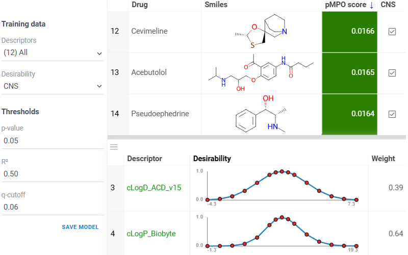
Available from
Chem -> Calculate -> MPO Score...: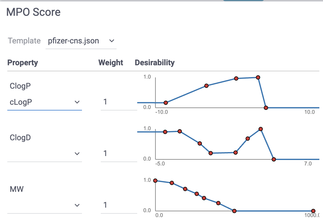
-
Pareto (multi-objective) optimization. Instead of collapsing objectives, identify the Pareto front: compounds for which no property can be improved without worsening another. Common in modern DDD pipelines and often paired with evolutionary algorithms or scalarization for ranking.
-
Active/Bayesian multi-objective optimization. Use surrogate models to propose new compounds that efficiently move the Pareto front (or a scalarized objective), reducing screening cost and focusing make/test cycles.
-
Desirability-based QSAR/MQSAR. Use the built-in predictive modeling capabilities to predict property desirabilities directly (or predict properties first, then score).
Pareto front
The Pareto front represents a set of non-dominated solutions in multi-objective optimization, where improving one objective necessarily degrades at least one other, revealing optimal trade-offs between conflicting goals. Use the Pareto front viewer to display these Pareto-optimal points on an interactive scatterplot:
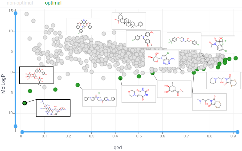
Launch an interactive Pareto Front application that enables real-time exploration of optimization results.
Generative chemistry
Generate novel compounds optimized for specific properties using Reinvent4. For details, see the Reinvent4 package docs.
Utilities
Datagrok offers multiple ways to transform and enrich your data. For example, you can link tables, extract values, or add metadata to annotate your dataset with experimental conditions or assay results. You can also use chemical scripts to execute operations on chemical data, including calculation of fingerprints and descriptors, toxicity prediction, and more.
Calculators
Molecular descriptors and fingerprints
Datagrok supports the calculation of different sets of descriptors and fingerprints:
- Lipinski, Crippen, EState, EState VSA, Fragments, Graph, MolSurf, QED. See this reference article for additional details.
- RDKFingerprint, MACCSKeys, AtomPair, TopologicalTorsion, Morgan/Circular. See this reference article for additional details.
For individual molecules, descriptors are calculated in real-time and presented in the Descriptors info pane (Context Panel > Chemistry > Descriptors), which dynamically updates as you interact with a chemical structure (e.g., upon clicking, modifying, or sketching a molecule.) You can also calculate descriptors or fingerprints for the entire column by choosing the corresponding option from the Chem > Calculate menu.
Molecule identifier conversions
Datagrok supports the conversion of various molecule identifiers, including proprietary identifiers, allowing you to work with multiple data sources and tools. For example, you can convert a SMILES string to an InChI and vice versa.
Supported data sources
| actor | drugbank | lipidmaps | pubchem |
| atlas | drugcentral | mcule | pubchem_dotf |
| bindingdb | emolecules | metabolights | pubchem_tpharma |
| brenda | fdasrs | molport | recon |
| carotenoiddb | gtopdb | nih_ncc | rhea |
| chebi | hmdb | nikkaji | selleck |
| chembl | ibm | nmrshiftdb2 | surechembl |
| chemicalbook | kegg_ligand | pdb | zinc |
| comptox | lincs | pharmgkb |
For individual molecules, the conversion happens automatically as you interact with molecules, and the Context Panel shows all available identifiers in the Identifiers info pane (Context Panel > Structure > Identifiers). You can also convert the entire column by choosing the corresponding option from the Chem > Calculate menu.
To run programmatically, use the #{x.ChemMapIdentifiers} function.
Curation
Datagrok supports chemical structure curation, including kekulization, normalization, reorganization, neutralization, tautomerization, and the selection of the main component.
How to use
To perform chemical structure curation:
- Navigate to Menu Ribbon > Chem > Transform > Curate.
- In the CurateChemStructures dialog, select from the available options and click OK. This action adds a new column containing curated structures.

Mutation
You can generate a dataset based on the preferred structure.
How to use
To perform chemical structure mutation:
- Navigate to Menu Ribbon > Chem > Transform > Mutate.
- In the Mutate dialog, draw or paste the desired structure and set other parameters, including the number of mutated molecules. Each mutation step can have randomized mutation mechanisms and places (select the Randomize checkbox).
- Click OK to execute. A new table with mutated structures opens.
Virtual synthesis
You can use the Chem: TwoComponentReaction function to apply specified chemical reactions to a pair of columns containing molecules in a virtual synthesis workflow. The output table contains a row for each product yielded by the reaction for the given inputs.

How to use
- Open the Two Component Reaction dialog by executing the
Chem: TwoComponentReactionfunction in the Console. This opens a parameter input dialog. - In the dialog:
- Select the reactants to use.
- Enter reaction in the filed provided.
- Choose whether to combine the reactants from two sets, or sequentially, and whether to randomize, by checking or clearing the Matrix Expansion and Randomize checkboxes.
- Set other parameters, such as seed, the number of maximum random reactions.
- Click OK to execute.
Customizing and extending the platform
Datagrok is a highly flexible platform that can be tailored to meet your specific needs and requirements. With its comprehensive set of functions and scripting capabilities, you can customize and enhance any aspect of the platform to suit your chemical data needs.
For instance, you can add new data formats, apply custom models, and perform other operations on molecules. You can also add or change UI elements, create custom connectors, menus, context actions, and more. You can even develop entire applications on top of the platform or customize any existing open-source plugins.
Learn more about extending and customizing Datagrok, including this cheminformatics-specific section.
Chemical scripts
Chem package comes with several scripts that can be used either directly, or as an example for building custom chemical functions in languages such as Python (with RDKit) or R. These chemical functions can be integrated into larger scripts and workflows across the platform, enabling a variety of use cases such as data transformation, enrichment, calculations, building UI components, workflow automation, and more. Here's an example:
- Script
- Script output
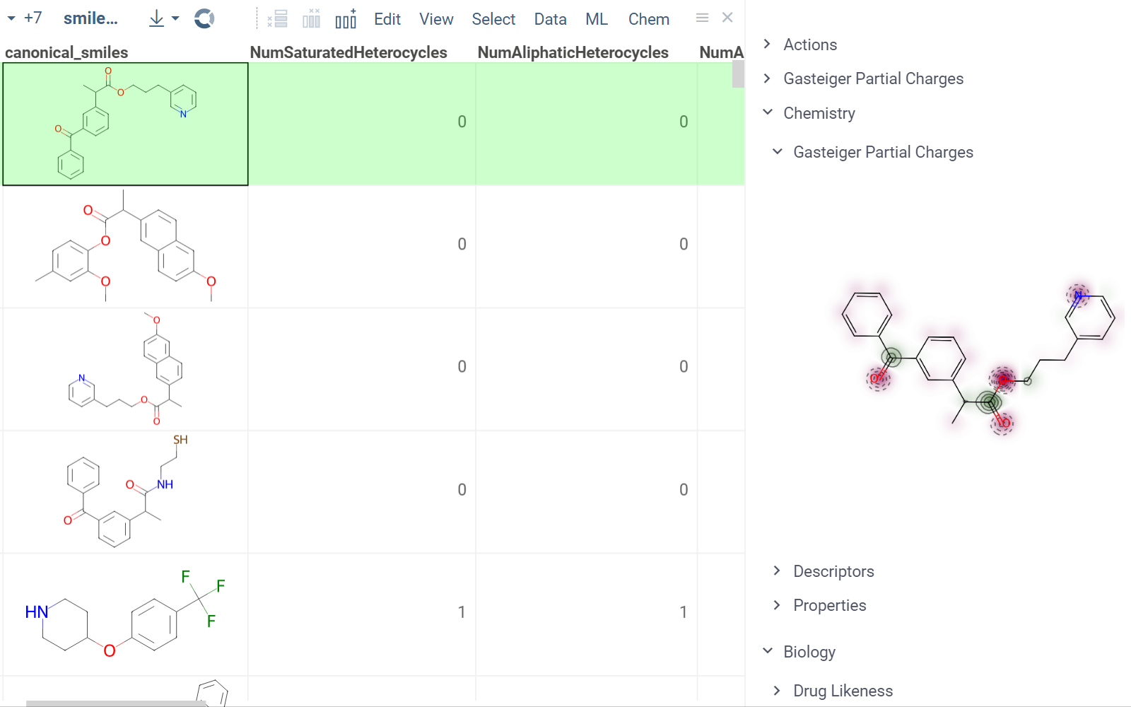
- Script output in info pane
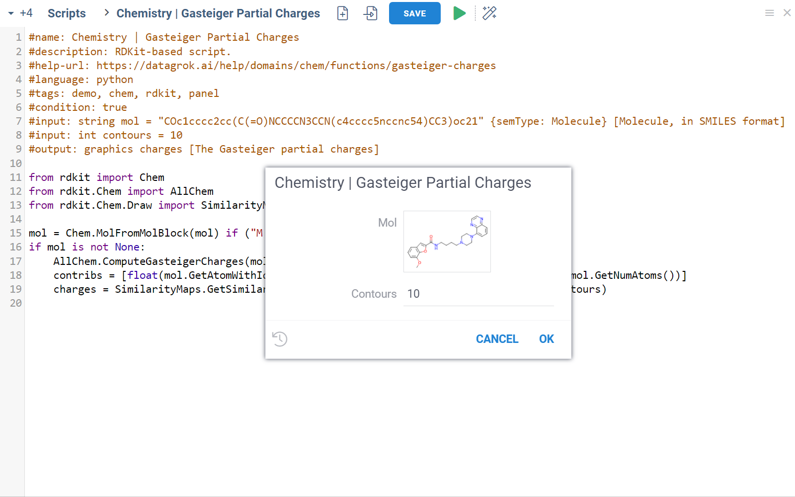
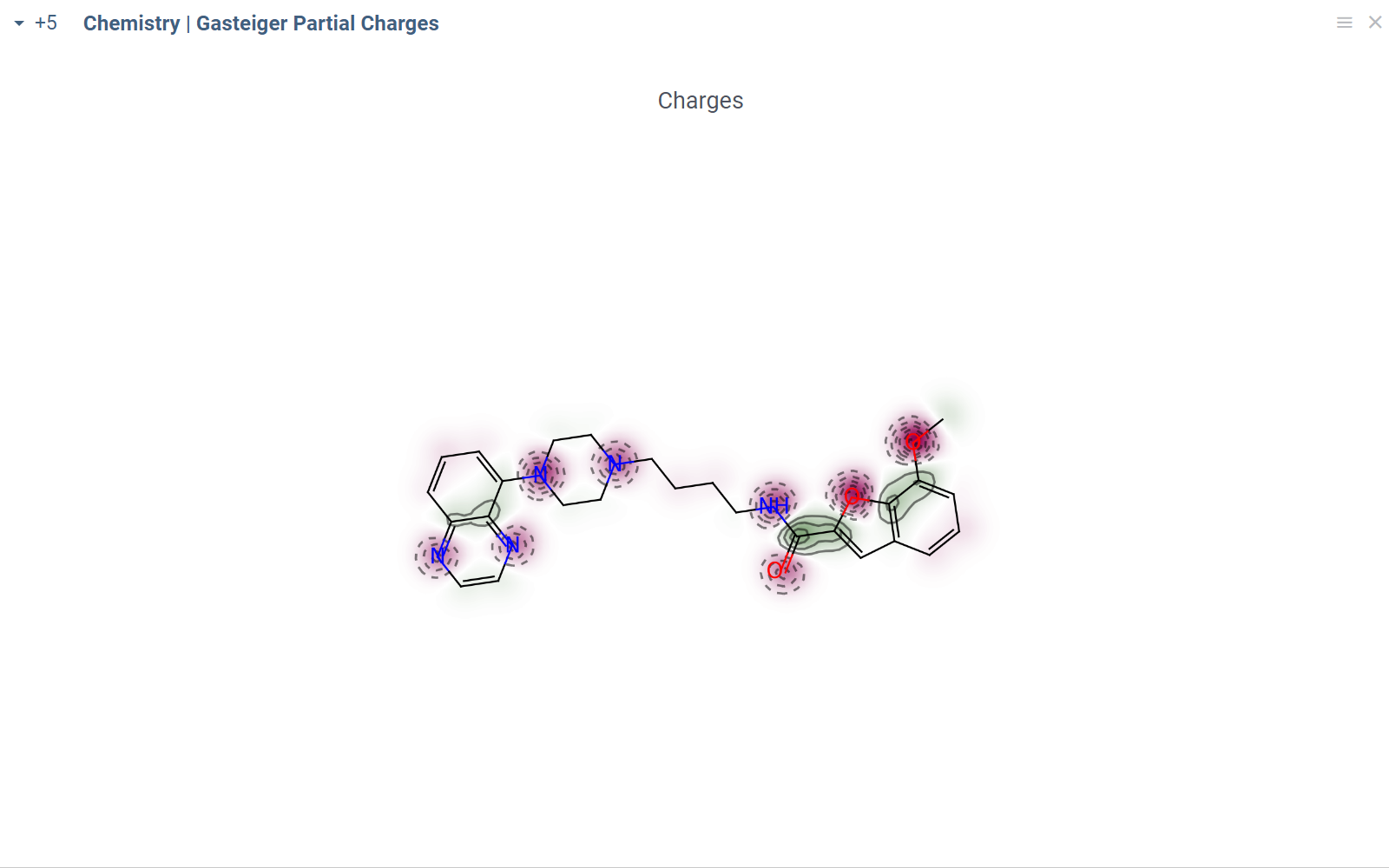
In this example, a Python script based on RDKit
calculates and visualizes Gasteiger partial charges. When you run the script
explicitly, Datagrok shows a dialog for sketching a query molecule and
visualizes the results. In this case, however, the script is also tagged as a
panel. This instructs Datagrok to show the results as an interactive UI
element that updates dynamically for the current molecule.
To view the chemical scripts you've created or those shared with you, open the Scripts Gallery (Functions > Scripts) and filter by the tag #chem. You can search for individual scripts and use the Context Panel to view details, edit, run, manage, and perform other actions for the selected script.
For a full list of chemical scripts, along with details on their implementation and associated performance metrics, see Chemical scripts. To learn more about scripting, see Scripting.